Reward

Reward is a key element in reinforcement learning, as it provides artificial intelligence (AI) with feedback regarding its performance, signaling whether its performance is correct or, on the contrary, leaves much to be desired. It should be noted that rewards are obtained only in terminal states, such as the end of a chess game. However, the number of non-terminal states is usually much larger, which requires correctly evaluating the value of the current state.

One method to carry out this evaluation involves evaluating the terminal states that the AI could reach through alpha-beta pruning, presented in the previous chapter. However, due to the immensity of the search tree, this strategy is not feasible. In the previous chapter, a solution to this problem was also discussed: the use of a heuristic. In this context, an analogous procedure will be applied, in which the heuristic will be calculated from the reward. This value will be called “expected reward”.

Direct calculation of the expected reward is not viable for the reason previously mentioned. However, it is possible to obtain approximations. These will be calculated through the simulation of numerous episodes, a generic term used in reinforcement learning to refer to all game matches, such as chess games. The initial estimate improves as more episodes are performed, refining the estimate of the expected reward.

To determine the expected reward, it is necessary to sum all the rewards obtained in subsequent states until the conclusion of the episode. In the case of chess, this process is simplified since the reward is zero in all non-terminal states. Additionally, a “discount” can be applied to the reward, which means that the longer it takes to obtain a reward, the lower its value will be. Thus, a reward of 1 obtained in the current state will have more value in the expected reward than a reward of 1 obtained three states later.

Below is an example to solidify these concepts. The 2-dimensional Grid game shows the game in question.

The objective of the game is to guide the black piece to the dark gray square. Upon reaching the dark gray square, a reward of 1 is obtained. The piece can move up, down, right or left. If these movements lead to a position outside the board, the episode ends with a reward of -0.5. Therefore, the piece must reach the dark gray square through a specific path. Since the piece does not know this path, the agent will have to discover it from the rewards obtained. Once an episode ends, the black piece returns to the initial position.

Initially, a run through the game is performed. The path followed is shown in the first Grid run.

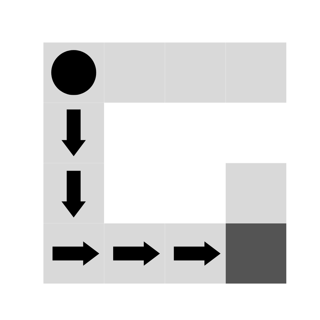
With this path, the game is successfully completed. Therefore, all states will receive a positive reward. In this case, a discount factor $\gamma$ of 0.99 will be used, which means that the expected reward of the next state will be reduced by 0.99.

With this discount factor, the expected reward for all the states through which the agent has passed can be easily calculated. The expected rewards after the first run show the result of these calculations.

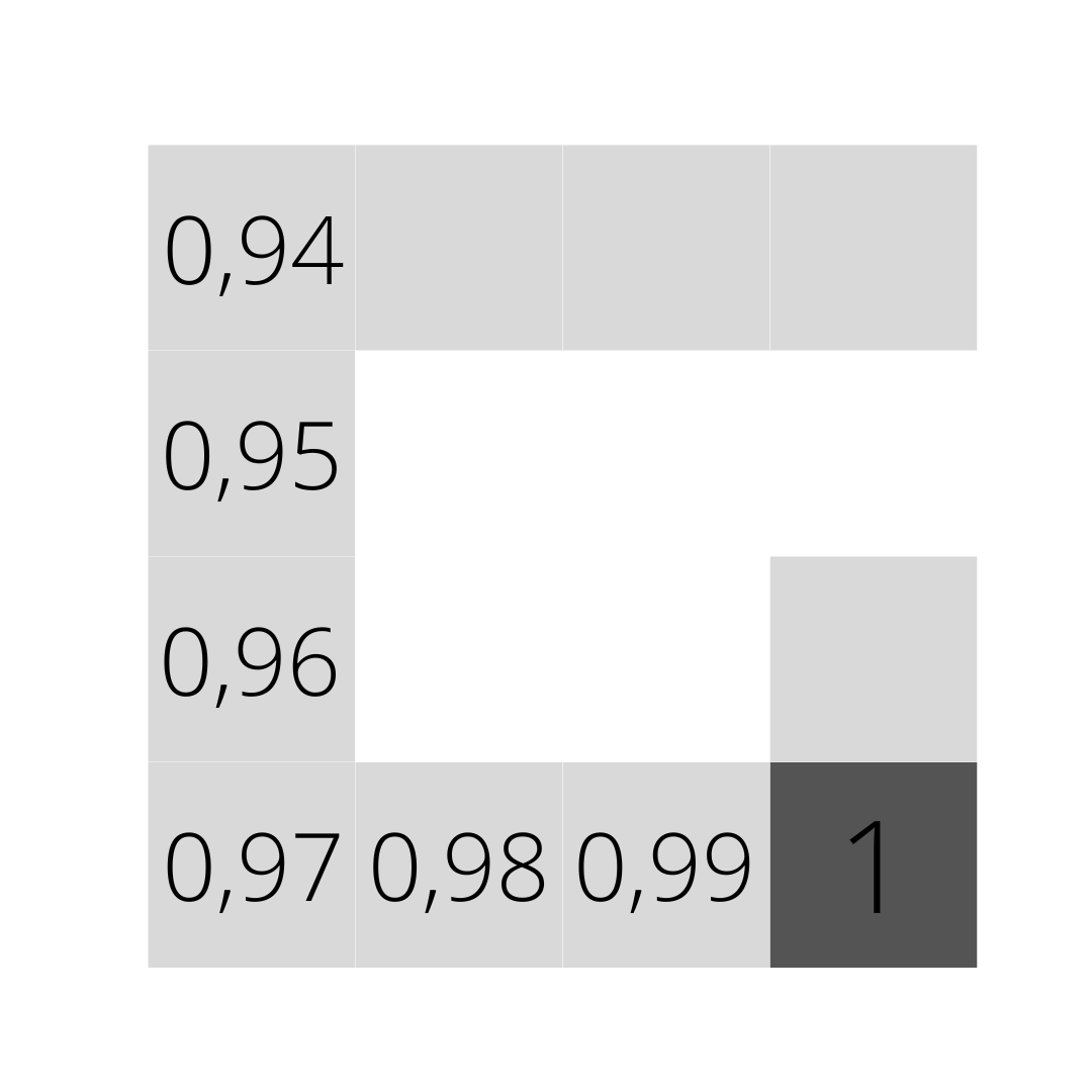
We start with the terminal state, which has a reward of 1. We proceed to the penultimate state, multiplying the reward of the final state by 0.99 and adding the reward of this new state (in this case 0). In this way, the expected reward of this state is obtained. This process is repeated until reaching the initial state, which has a reward of 0.94 (all values are rounded to two decimal places).

Another run is made through the Grid, but this time it will not be so successful and the piece will go off the path. The path followed is shown in the second Grid run.

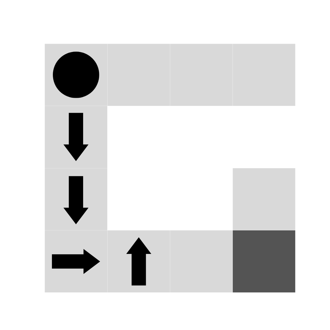
Now it is time to update the squares through which the piece has passed. Its new value will be calculated as the average of the expected rewards from the first and second runs for the squares that are included in both paths. The expected rewards after the second run show the final result of these calculations.

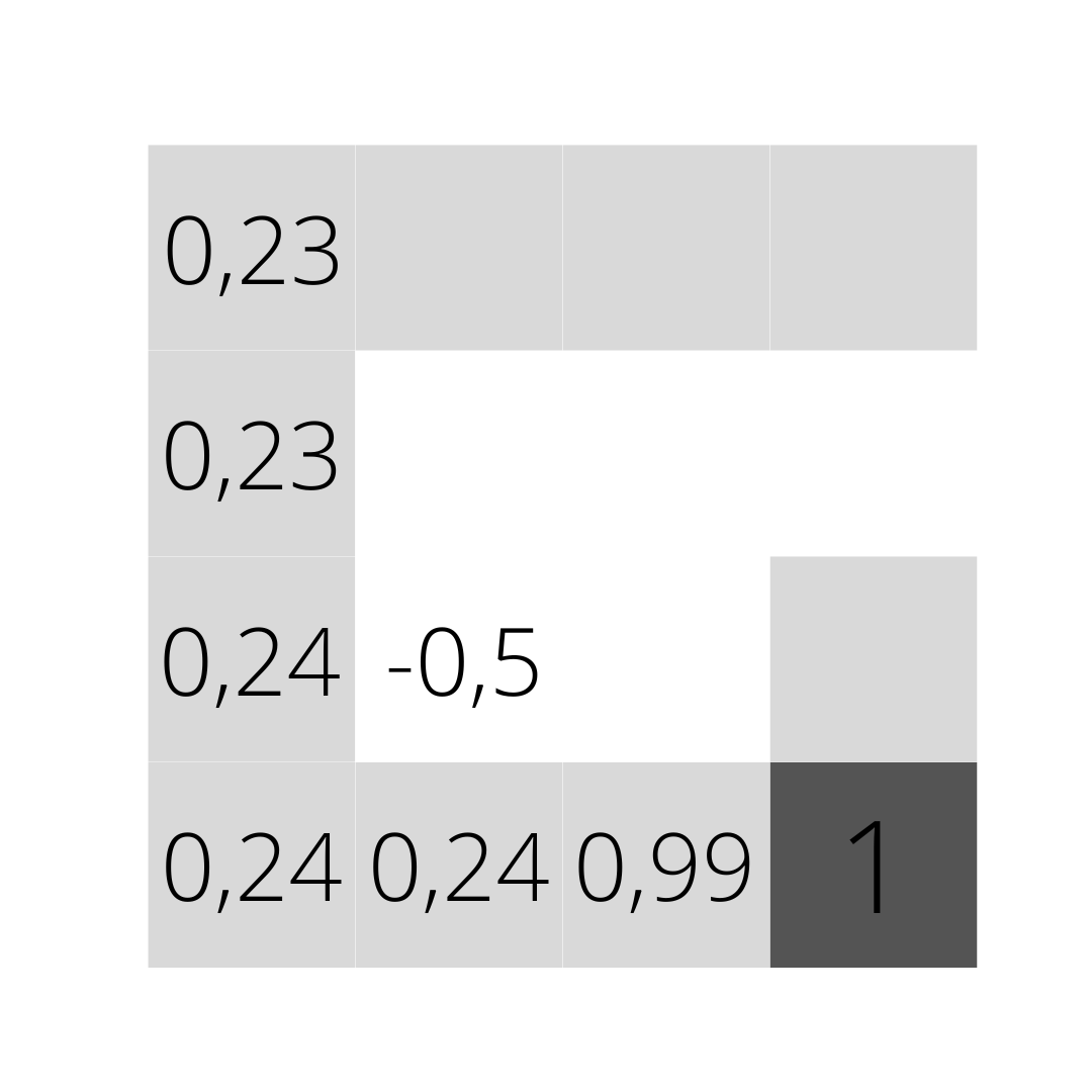
We start again from the terminal state (the square with value -0.5 which is where the piece deviated from the path) and each state is processed, calculating its new value as explained above. This process can be repeated as many times as necessary. Although the more it is repeated, the more accurate the values of each state will be, it must be taken into account that this involves a computational cost.

The game presented above is completely deterministic (it is known which state will be reached with each action), but in some cases, a given action could lead to different states according to a probability distribution. The problem with this type of game is that the process that has been followed previously would no longer be valid. However, it can be solved in a simple way by assigning values to the action taken in a specific state, that is, the value is known from the state and the action taken in that state.

Another aspect to consider is determining which path to take. In the previous case, the path has been random. This would be a random policy. The policy defines which action to take given a particular state. This topic will be addressed in the next section.