Board representation

After exploring the search mechanisms in artificial intelligence games, it is crucial to examine another essential component: the representation of the game board. This element fulfills two primary functions in the context of search. The first of these is the generation of all possible moves from the current position in the game. Secondly, it handles the transitions from one move to the next, that is, it provides the new position on the board based on the move and the previous state of the same. Both functions are invoked repeatedly in the game tree. Given the relevance of these operations and the fact that the quality of a move depends both on the depth of tree expansion and the time this entails, it is essential that both functions be implemented as efficiently as possible.

For an effective implementation of these functions, it is imperative to consider how the game board is represented in the computer’s memory. There are various methods for this, each with its own benefits and limitations. We can group these methods into three general categories: piece-centric methods, board-centric methods, and hybrid methods [Chessprogramming Wiki]. The nomenclature of these categories is quite descriptive.

Piece-centric methods focus on representing the pieces directly, maintaining lists or other data structures with the information associated with each piece and its position on the board. On the other hand, board-centric methods focus on examining each square of the board individually to determine if it contains a piece and, if so, what type of piece it is. Finally, hybrid methods are those that combine aspects of both approaches.

Apart from the information of the board or pieces themselves, it is necessary to store additional information, such as the possibility of castling, the number of times the current position has been repeated, the number of moves without captures or pawn advances, among others. This type of information is relatively simple to represent, so not much emphasis will be placed on it, focusing more on the information of the board and pieces.

Before discussing the main techniques, it is necessary to establish the difference between pseudolegal moves and legal moves. Legal moves are all those that can be made in a position according to the rules of chess. Pseudolegal moves, on the other hand, include legal moves and those that cannot be made because they would leave the king under attack and, therefore, would be illegal according to the rules of chess. It is important to consider these groups separately because pseudolegal moves are easier to calculate compared to legal moves. Checking if the king is in check after a move implies a significant additional computational cost. To solve this problem, moves can be generated one by one, verifying if the king is left in check before making each move. Another option is to allow the pseudolegal move and, if the opponent has the opportunity to capture the king on their turn, that move is invalidated.

Next, we will begin with a brief summary of the main board representation techniques and then delve deeper into the most relevant ones:

• 2D Array: This board-centric method employs an $8 \times 8$ matrix where a value of 0 in a matrix position indicates that the corresponding square is empty. Each piece type is assigned a number; for example, pawns are assigned a 1, knights a 2, etc. If the piece is white, it is assigned a positive value; if it is black, a negative value. For example, if the bishop is assigned the number 3, a white bishop would be 3 and a black bishop -3.
• Piece list: This piece-centric technique maintains a list of all pieces in play. Each entry in the list contains the piece type, color, and the square on which it is located. For example, for a white bishop on square a4, the list will store an entry with the bishop, the white color, and square a4.
• Bitboard: This is the most commonly used representation and is board-centric. The main idea is to use bitsets A bitset is a simple data structure used to represent a set of elements, such as numbers or boolean values. It works by assigning a single bit (0 or 1) to each element in the set, allowing membership verification of an element in constant time. to represent $8 \times 8$ matrices. Since only 0s and 1s can be used, it is necessary to use one matrix for each piece type and color, which gives a total of 12 matrices. If a piece’s matrix has a 1 in a certain position, that square will contain that piece; if, on the contrary, it has a 0, there will not be a piece of that type on that square. Despite the fact that it may seem less efficient than the 2D matrix, having to use 12 matrices instead of one, this method has a series of advantages that will be discussed later.
• Attack vectors: This board-centric method represents the movements of pieces as vectors. Each piece is assigned a series of vectors according to its movement. For example, the queen combines the vectors of rooks and bishops. Thanks to the vectors, moves can be generated. When moves are generated, the piece moves using the vector until it finds an obstacle, and all the squares it has passed are considered as moves. For the knight, pawn, and king, it will be necessary to consider their peculiarities in movements.

Of all the techniques described, we will only address the bitboard technique in depth. This is because one of its variants, the magic bitboard, is one of the most widely used today. In addition to those mentioned, there are many more representations that work better or worse depending on the structure of the module itself and even on the programming language used to create it.

The Bitboard concept relies on the use of so-called bitsets. A bitset is a set of bits, each bit can take only two values: 0 or 1. In this way, it allows us to represent whether a square is occupied by a piece type (including color) or not.

One of the most relevant attributes of bitsets is their ability to be represented by an integer number. This is particularly useful in situations where we need to manipulate or represent information in the form of bits.

Let us consider a four-bit bitset as an example. In this case, the number 3 is represented as “0011”. Therefore, a four-position bitset can represent any number from 0 to 15. We can convert a bitset to its numerical equivalent using the formula:

$$n = \sum_{i=0}^{k-1} b_i * 2^i$$

In the formula, $n$ is the number in decimal format, $k$ is the number of bits the bitset has, and $b_i$ is the bit at position $i$ counting from the right. Thus, the first bit would be the last, the second bit would be the penultimate, and so on. Consequently, a bitset of $k$ positions can represent numbers from $0$ to $2^k-1$. This implies that a bitset can represent $2^k$ numbers in total, although starting at $0$ it does not include the number $2^k$.

Making use of this principle, let us consider the application in the game of chess. We know that a chessboard has 64 squares, so we would require a bitset of size 64 for its representation. Fortunately, modern computers are optimized to work efficiently with 64-bit integers, as they support them natively. Therefore, with just 12 integers, we could represent all possible chess boards! In terms of efficiency in memory usage (measured in terms of bits used), this is not necessarily the best option, but the true value of this method lies in its ability to quickly generate possible moves from a given position through the use of logical operations.

Computers perform two types of basic operations: arithmetic and logical. Arithmetic operations are standard operations such as addition, subtraction, multiplication, and division, while logical operations operate on Boolean algebra. This type of algebra only contains two values, 0 and 1, and constitutes the fundamental basis of computing. Arithmetic operations normally require a large number of logical operations for their execution, so logical operations are usually faster This refers to digital electronics.

Logical operations are usually performed on one or two variables, although they are easily extensible to a greater number of variables. To represent these operations, so-called logic gates are used. These take one or more variables as input and generate a single output. Both the variables and the output can take the values 0 or 1.

The main logic gates for one variable are those shown in Table 1.

Values	NOT	Identity
0	1	0
1	0	1

Single-variable logic gates

The NOT logic gate inverts the value of the input. If the input is 0, the output will be 1 and vice versa. On the other hand, the identity gate simply leaves the input value unchanged.

Next, let us consider two-variable logic gates, which are somewhat more complex but can be extended to more than two variables. Table 2 shows the main two-variable logic gates.

Values	OR	AND	XOR
00	0	0	0
01	1	0	1
10	1	0	1
11	1	1	0

Two-variable logic gates

The OR logic gate produces an output of 1 whenever at least one of the inputs is 1. This behavior is maintained if extended to more than two variables: the output will be 1 if at least one of all the variables is 1.

The AND logic gate produces an output of 1 only when all inputs are 1. This logic also applies when there are more than two inputs.

To conclude our exploration of logic gates, the XOR gate represents a peculiar use case. It can be conceived as a more “strict” version of the OR gate. Similarly, the XOR gate operates just like an OR gate, with a significant exception: in the case that all inputs are 1, the output will be 0.

When we expand this gate to more than two inputs, two methods can be followed: it will return 1 if the number of inputs that are 1 is odd, and it will be true if and only if there is exactly one input that is 1. However, it is important to note that neither of these approaches is considered universally applicable. From an electronic perspective, an XOR gate with more than two variables is not generally implemented.

There are several other logic gates besides those already mentioned. These can be derived through the combination of the previously described gates. NAND and NOR gates deserve special mention. They are the result of combining the OR and AND gates with a NOT gate, respectively. In other words, they take the value of the OR and AND gates and then invert it. The importance of these gates lies in their consideration as “universal”. This means that, using exclusively NAND or NOR gates, we can recreate all other logic gates, even those with a single input. These operations play a fundamental role in making bitboards efficient.

To illustrate these concepts, we will show an example of how a chessboard is converted to its bitboard representation.

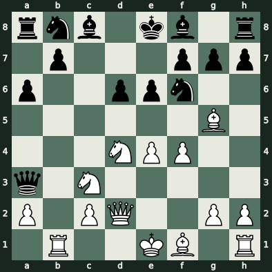
In this representation, the bits originate in the lower right corner, which implies that bit 0 (located at the end) corresponds to square h1. The bits are assigned by columns, and once all the bits of a column have been assigned, it proceeds to the next row starting from the initial column. Therefore, bit 1 corresponds to g1, bit 2 to f1, and bit 8 to h2, and so on.

To begin, we will represent the white pawns. Every 8 bits will be separated into different lines to simplify reading. The resulting representation would be as follows:

00000000
00000000
00000000
00000000
00001100
00000000
10100011
00000000

Rows 4 and 2, where the white pawns are located, are the only ones that contain ones. Next, we show another example with the black rooks.

10000001
00000000
00000000
00000000
00000000
00000000
00000000
00000000

The black rooks remain in their initial positions. This same procedure would be used to represent the rest of the pieces.

To generate moves, a highly efficient technique known as magic bitboards is employed. This technique is used to calculate the moves of bishops and rooks, and therefore, those of the queen. Knights, the king, and pawns are simpler to calculate, so it is not necessary to use this technique with them. This is because the movements of these pieces are not “obstructed” by other pieces.

The magic bitboards technique consists of multiplying the current board, represented by its bitset, by certain “magic numbers”. For each position of a bishop or rook, and an arrangement of pieces that can block its path, there is a magic number that, multiplied by the bitset that contains all the pieces on the board (this is calculated by doing an OR between all the bitsets), provides us with all possible moves of the bishop or rook in a new bitset. Calculating these magic numbers involves a high computational cost, but it only needs to be done once and serves for any position. This is the reason why this technique offers such remarkable performance.

To summarize, there is a multitude of techniques that allow chessboards to be represented, focusing mainly on move generation and transitions between different game states. One of the most prominent and widely used techniques is that of magic bitboards. This method is known for its exceptional efficiency in terms of performance and speed.

In addition to magic bitboards, there are other board representations that are more suitable for certain specific applications. For example, the one-hot encoding method, which shares similarities with the bitboard representation, and the HalfKP representation, are both widely used in neural network contexts due to their particular properties.

On the other hand, FEN (Forsyth-Edwards Notation) notation is widely used to store and retrieve chessboard positions, given its ability to concisely represent the complete state of a game.

It is important to note that all these techniques will be presented in greater detail in later chapters of this book, giving the reader a deeper understanding of their characteristics and applications in different contexts.