The king's marches

The king’s ways

In this chapter, the question of how many routes a chess king can take, starting from one specific square to another, using the minimum number of moves will be addressed. Although this question may seem simple at first glance, it will reveal itself as a more complex inquiry than might initially be expected. As an illustration of this, let us consider a standard 8x8 chessboard and estimate how many moves would be required to reach each square from an initial king position on square e5.

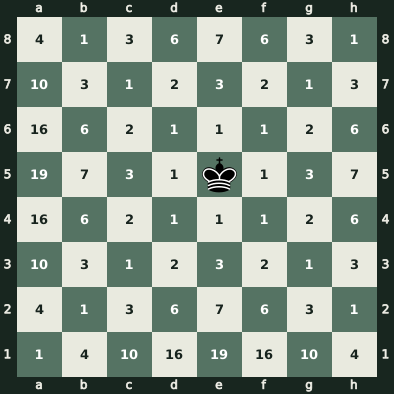
By observing the figure, several interesting conclusions can be drawn regarding how many routes exist to reach each square. First, it is worth noting that in the squares adjacent to the king - whether horizontally, vertically or diagonally - there exists only one possible route to arrive in the minimum number of moves.

In addition to the adjacent squares, there are others marked with the number one, indicating that there is only one way to reach that square. These are the squares that are on the king’s diagonals. Since to reach these squares one must always make diagonal moves, it is consistent that there is only one route. More generally, it is observable that the farther a square is from the king, the greater the number of available routes to reach it.

Another interesting question to consider in relation to this topic is the minimum number of moves that the king needs to make to reach a specific square. This problem is considerably simpler than the previous one and can be solved using a simple formula. However, having knowledge of this minimum number of moves can provide very valuable information to solve the original question.

To simplify the understanding of this problem, we can begin by examining the squares closest to the king. First, the square on which the king is located has a distance of zero. The squares adjacent to the king - whether horizontally, vertically or diagonally - will have a distance of one. With respect to the other squares, those adjacent to the squares with a distance of one will have that distance plus one, that is, a distance of two. By calculating the distance of the squares adjacent to those whose distance is already known, it will be possible to determine all distances. The distance map for an 8x8 board illustrates the distance to each of the squares, considering the king situated on the same square on a board of equal size.

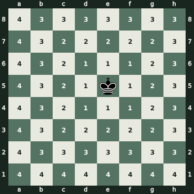
In addition to the strategy mentioned above, it is also possible to resort to a direct formula that, knowing the position of the king and the coordinates of the target square, provides the minimum number of moves necessary for the king to reach it. The formula is as follows:

$$\max(\abs{r_0-a_0},\abs{r_1-a_1})$$

Where $r = (r_0,r_1)$ are the coordinates of the king, where $r_0$ represents the row and $r_1$ the column, and $a = (a_0,a_1)$ the coordinates of the square whose distance is to be calculated, with $a_0$ being the row and $a_1$ the column of said square. In the case of rows, the conversion is direct, but for the column, the numerical conversion of the letter must be used. That is, “a” becomes 1, “b” 2, and so on.

It is natural to wonder where this formula comes from and why it works. First, it can be verified that for the previous board, correct results are obtained on all squares, which suggests that the formula is reliable. To guarantee its validity, a mathematical proof would be necessary, but since this exceeds the scope of this book, you will have to trust my word.

The intuition behind this formula is based on the idea that the king takes the same time to move to an adjacent square, even if it is diagonally located. This does not happen with more common distances, such as Euclidean distance (Pythagorean Theorem) or Manhattan distance (where moving to a diagonally adjacent square would have a cost of 2). In our formula, what happens is that it calculates how many rows and columns of difference exist, and since the king can move diagonally, the distance turns out to be the maximum value between the number of rows and columns that separate the two coordinates. This distance is known as the chessboard distance or Chebyshev distance.

Returning to the main problem after this brief digression, it is necessary to find a formula that allows us to calculate how many routes exist to reach a square in a minimum number of moves. First, we must focus on a specific square, which in this case will be d1. The route count for square d1 shows how many routes exist to reach that square, along with a revealing observation.

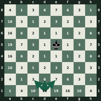
The arrows in the figure point to three adjacent squares, and curiously, the sum of the values of these squares equals the value of square d1. The question might arise: why choose these three adjacent squares instead of the other adjacent squares? To answer this question, it would be useful for the reader to look again at the distance map.

Square e1 is at a distance of 4 squares from the king, while the adjacent squares analyzed are at a distance of one unit less, that is, 3. From this scenario, we can generalize that the number of routes to a given square will be the sum of the number of routes to the adjacent squares that are at a distance of one unit less. If the reader is skeptical about this statement, they can proceed to verify it in the figures previously shown.

The route-count calculation for square d1 illustrates the process of continuously applying this strategy until reaching the final value.

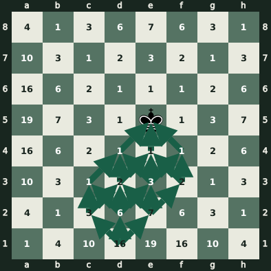
Therefore, to calculate the number of paths to a specific square, we must know how many routes exist to the adjacent squares closest to the origin square. This, in turn, implies that we would have to perform this same calculation for these adjacent squares using the squares adjacent to them, and so on until reaching the initial square. In this last case, to facilitate the calculations, we establish that there is a single way to go to the initial square from the initial square itself. With this information, we can define the following mathematical formula that allows executing the entire described process:

$$f(x, k) = \begin{cases} 1 \text{,} & \text{if } x = k \\ \sum_{c \in C_x} f(c, k) \text{,} & \text{if } x \neq k \end{cases}$$

Where $f(x, k)$ is the function that indicates the number of routes from square $k$ to square $x$ and $C_x$ are all the adjacent squares closest to square $x$. Therefore, the formula will return 1 if we are on the initial square and, otherwise, will calculate the value by adding the values obtained by the functions on the adjacent squares.

After analyzing the formula, we can notice that it contains recursion; the upper part of the piecewise function would correspond to the base case, while the lower part would be the recursive case. Being a recursive function, it would be relevant to analyze the number of recursive calls that would be necessary in the case of a computational treatment of the function. Returning to the route-count calculation, we see that some values are calculated several times, which obviously is a waste of time. Regarding this point, we can analyze the number of recursive calls using the theory seen in the previous topic. In the example analyzed above, we could see that, depending on the square, there can be 1, 2 or 3 recursive calls if it is not the base case and, as we already know, the worst case must be chosen, where there are up to three recursive calls. Additionally, we must consider that, in this case, the size of the problem will not be the size of the board, but the distance between the analyzed square and the king. Below, the formula that gives the complexity of the algorithm is shown.

$$3^{\max(\abs{x_0-k_0},\abs{x_1-k_1})} \in O(3^n)$$

Returning to the problem of the numerous recursive calls for the number of squares we process, the astute reader will realize that some arrows point to the same square and this indicates that we calculate the value of the same square several times, which clearly is not efficient. Wouldn’t there be some way to avoid this? The answer is yes, when the value of a square is calculated, its value can be stored in a vector or matrix, depending on the situation, to avoid having to recalculate it. This procedure is known as dynamic programming.

Dynamic programming vs. the king’s marches

The concept of “dynamic programming” can be somewhat mysterious at first glance, and one might wonder: what is the origin of this peculiar name? The answer to this question is quite unusual. Richard Bellman, the inventor of the term, chose it strategically to avoid having his research canceled. Aware that an attractive and vague name like “dynamic programming” would make any cancellation attempt difficult, he opted for this designation.

With the origin of the name clarified, it is time to explore the essence of dynamic programming and its usefulness in problem solving. The main appeal of dynamic programming lies in its ability to simplify high-complexity problems, especially those with exponential or higher complexities, and convert them into polynomial complexity problems. This is possible thanks to a fundamental characteristic of dynamic programming: the ability to store and reuse already calculated partial solutions, thus avoiding the cost of unnecessary recalculations. Despite being a simple concept, its effectiveness is extraordinary and has significant applications in a wide range of problems.

Now that we have examined the fundamental principle of dynamic programming, we will delve into a practical case to appreciate its effectiveness in reducing the number of recursive calls. We will start with the board shown in the initial dynamic-programming board, focusing on square e1, which has been used previously.

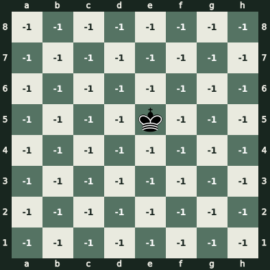
By examining the board, it is noted that all squares have a value of -1. This value is a marker that indicates that the distance to that square has not yet been calculated. In the first resolution phase, we focus on calculating the different ways we can reach square c2.

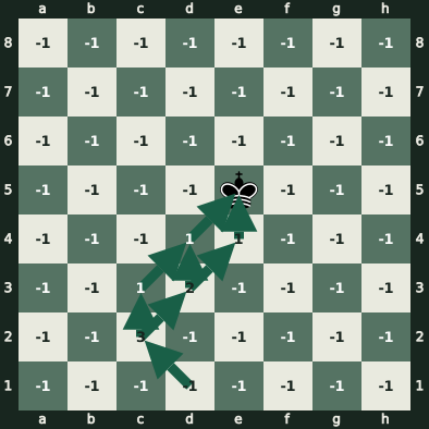
In this first phase, the value of square c2 has been calculated, which turns out to be 3. Additionally, the values of all the squares necessary to obtain the value of c2 have been determined. To avoid redundant calculations, all these values are stored in a matrix, preparing them to be reused in future operations. In fact, the need for this practice has already been demonstrated in this phase, since the value of square d4 has been required both for the calculation of square c3 and for square d3.

After concluding the first phase, we embark on the second, where the value of square d2 is calculated. This calculation corresponds to the second recursive call required to determine the value of square d1. The calculation procedure for this phase is illustrated in the second dynamic-programming phase.

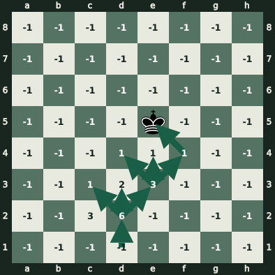
In this second phase, even more intensive use is made of the already calculated values, especially those that were determined in the previous phase, such as squares d3 and e4.

Finally, we reach the final phase, in which we finally calculate the value of square d1. This calculation can be seen in the final dynamic-programming phase.

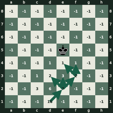
The problem resolution process intensifies even more in its use of the values of previously calculated squares. In general terms, as the algorithm progresses, more calculations can be saved. At this point, we have achieved such efficiency that it is no longer necessary to reach the base case.

To summarize everything discussed so far:

The term “dynamic programming” was coined by Richard Bellman as a strategy to protect his research from possible cancellations. This method is characterized by its ability to simplify high-complexity problems into polynomial complexity problems. This is achieved through the storage and reuse of already calculated partial solutions to avoid recalculations.

In a practical example, we analyzed how dynamic programming was applied to a chessboard. In the first phase, the number of ways to reach square c2 was calculated, storing the values of the squares necessary for this calculation. The second phase involved calculating square d2, making intensive use of the values already determined in the previous phase.

Finally, in the last phase, the value of square d1 was calculated, highlighting the efficiency of dynamic programming, as more calculations were saved as the algorithm progressed. This procedure proved so effective that it was not even necessary to reach the base case. In essence, dynamic programming proves to be an exceptionally effective and economical approach for solving complex problems.