The minimax algorithm

Introduction

The operation of the minimax algorithm is intrinsically anchored to its denomination. This algorithm is used to identify the theoretically optimal move in any perfect information game — where all players have complete and shared knowledge of the game state — and zero-sum — where one player’s gains are balanced by the other(s) player’s losses. This algorithm presupposes that both the player using it and the opponent will make optimal moves. This is where the algorithm’s name becomes relevant: the player will select the move that maximizes their benefit, while the opponent will choose the move that minimizes the player’s benefit.

These maximization and minimization processes unfold at all levels of the game tree, which was broken down in a previous section. Each state of the tree is classified by its level, which is defined as the number of transitions required to reach that state from the initial or root state. Therefore, the root is identified as level 0, states directly linked to it as level 1, and so on.

In the even levels of the game tree, the player maximizes their advantage by choosing the most beneficial move, while in odd levels, minimization comes into play when the opponent attempts to select the move that provides the least benefit to the player.

One last aspect to explain is how the valuation of each state is determined. Ideally, one could explore each branch of the tree until reaching a final state, and thus know the true valuation of each state. However, in practice, this exhaustive exploration is infeasible, so we resort to heuristics. At a predetermined depth level, the development of the game tree is stopped and the final states of each branch are evaluated with the heuristic. From these valuations, the valuations of the remaining states are calculated in a bottom-up process, until reaching the initial or root state of the game tree. Obviously, the minimax algorithm is employed for this process.

The concept of the minimax algorithm can be somewhat abstract at first glance, so a step-by-step example of its application is provided in the section below.

The first step is to calculate the values of the final states of the generated game tree (in this case, the states at the end of each branch), using the heuristic. This process is represented in the first generic Minimax step.

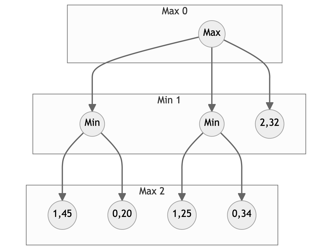
In the decision tree, those values that have already been determined are illustrated using their corresponding numerical value. On the other hand, nodes whose values have not yet been calculated will be represented as Max or Min, depending on whether their value will be the maximum or minimum of their respective child nodes. It is important to note that nodes whose values have already been calculated do not have child nodes, that is, they are not linked to any node at a lower level. In decision tree terminology, these nodes are called leaf nodes, making an analogy with the leaves of a tree in the natural world.

Once the heuristics of these final states have been calculated, we can proceed to determine the heuristic of the immediately adjacent level. To do this, we must take the minimum value of the states at the lower level, which corresponds to the minimization phase. For example, at the node located on the left of level 1, we will take $\min(1,45;0,2)$, here, the use of the semicolon is to avoid confusion with the comma used to separate decimal and integer figures, and we will obtain 0,2 as a result, since this value is less than 1,45. Following this process, at the central state of level 1, we select $\min(0,25;0,34)$ and obtain 0,25, since it is less than 0,34. Finally, the node located on the right at level 1, being a final state, already has a calculated value, so it is temporarily ignored. The second generic Minimax step illustrates the result of this process.

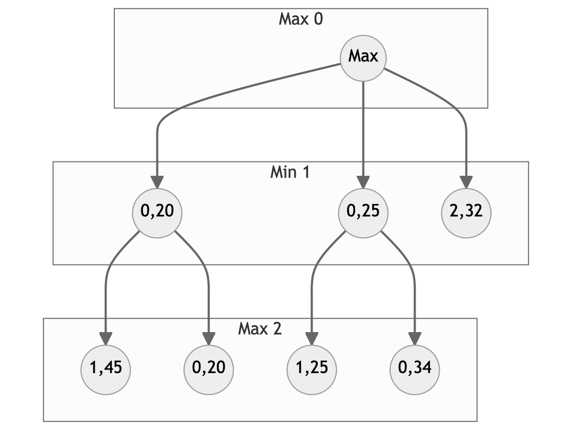
Now, we must carry out a maximization phase. That is, we need to obtain the maximum value of the lower adjacent states to the state located at level zero or initial state. Thus, we apply $\max(0,2;0,25;2,32)$, obtaining 2,32 as a result, since this value is greater than 0,2 and 0,25. Since this is the initial state, the Minimax algorithm has been completed. Therefore, we can determine that the best transition is the one that leads to the state with value 2,32. The third generic Minimax step shows the finalized game tree.

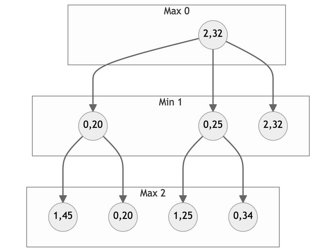
It is relevant to mention that not all final states are at the same depth level. In the previous example, the final state with value 2,32 is at level 1, instead of being at level 2, like the others. This can happen if the state with value 2,32 represents a final state in the complete game tree (that is, it cannot be expanded further from there) or it has been decided not to expand that node further. This latter technique is commonly used, since through an additional heuristic (which determines how beneficial it is to expand a state) one can decide whether it is valuable to continue expanding that state or to end the branch at that point.

After reviewing this simple general example, we can move forward to a more complex and realistic example in which the minimax algorithm is applied to a chess game.

Minimax algorithm applied to chess

Special considerations

Chess, as a specific case of minimax algorithm application, has some particularities. Most relevant is that the size of the chess game tree is immensely large, a fact that has been repeatedly emphasized. This motivates us to seek ways to reduce the number of states that are added to the simulated game tree used by the minimax algorithm. One strategy that has already been mentioned consists of using a heuristic that allows evaluating how “interesting” a state is to decide whether to explore it. This concept of “interesting” helps establish a priority in the expansion of states, since we are unlikely to have time to explore all of them to completion. When defining this heuristic, we should consider factors such as the level of the state relative to the initial state, the value of the heuristic that indicates the quality of a position, among others.

Finally, it should be noted that the expansion of this game tree will be limited primarily by available time. For example, in a game with limited time, the computer must return the best move it has been able to find in the brief time it has. Conversely, if the game allows more extensive playing time, the computer will have more time to find the best move, which will likely result in a better solution in the same position than in the previous case, since it has been able to expand the game tree more.

Example applied to chess

The Minimax chess game tree is presented, representing the sequence of moves in the example of minimax algorithm application to chess. The initial position corresponds to the start of a standard chess game, where White makes the move d4, followed by Black’s response with d5. From this position, White must make the decision to determine which move is best.

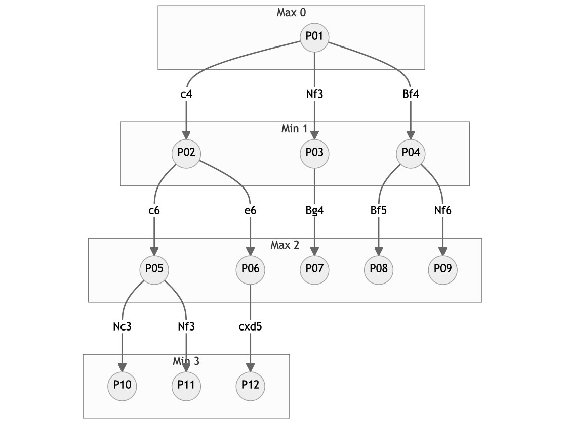
Each node of the tree represents a board position and the different branches indicate the possible moves that can be made from that position. The boards in the Minimax chess example show the boards corresponding to each position represented in the example of minimax algorithm application to chess.

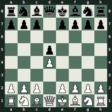
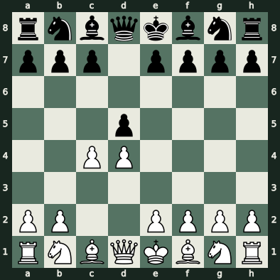
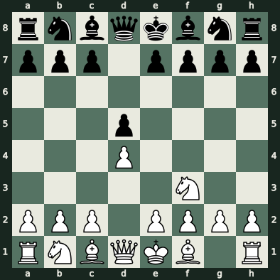
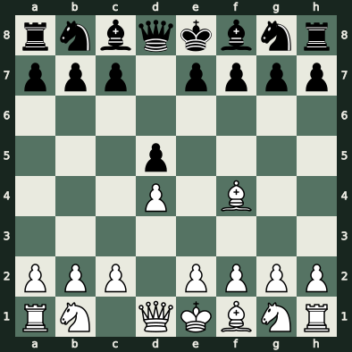
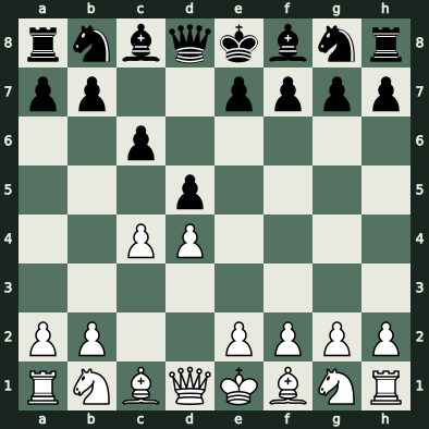
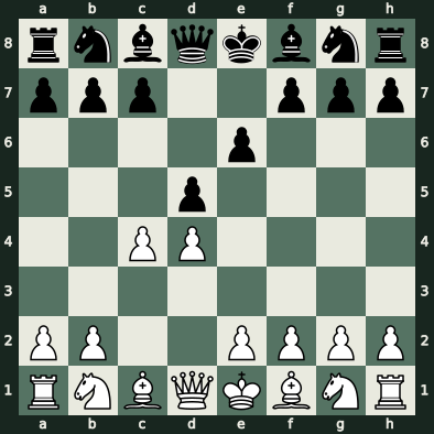
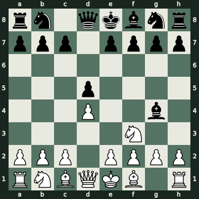
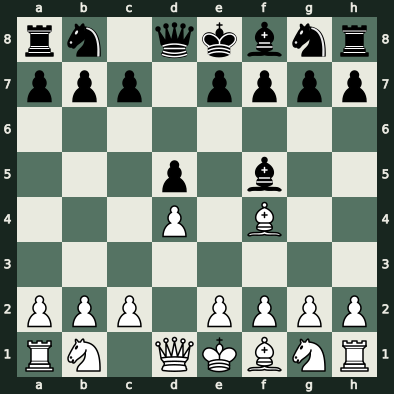
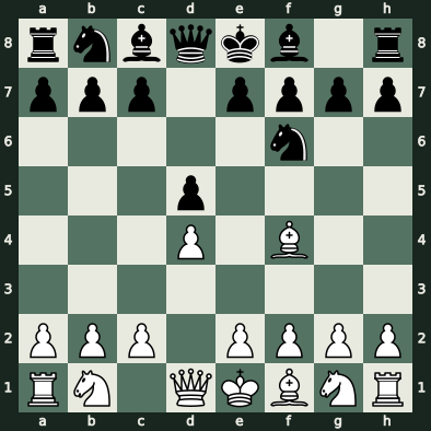
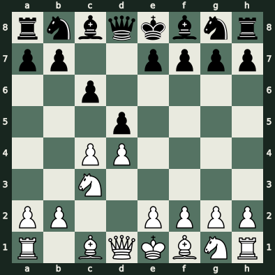
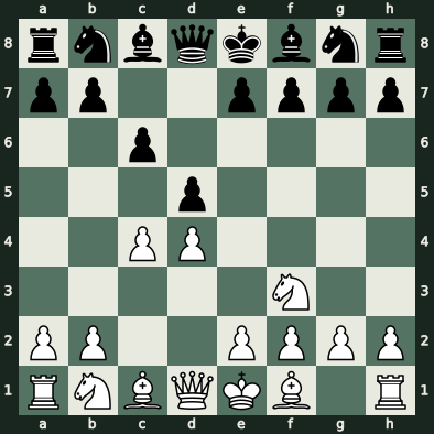
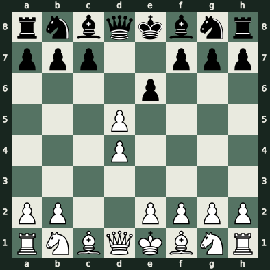
Once the game tree and corresponding positions have been obtained, one can proceed to the next phase of the Minimax algorithm, which consists of calculating the value of terminal positions. These positions refer to those that have no branches exiting from them, that is, no more moves can be made from them.

When calculating the heuristic of these terminal positions, a realistic approximation of the value of each position will be obtained. The result of this calculation will give rise to a new representation of the game tree, as shown in the first phase of the chess Minimax example.

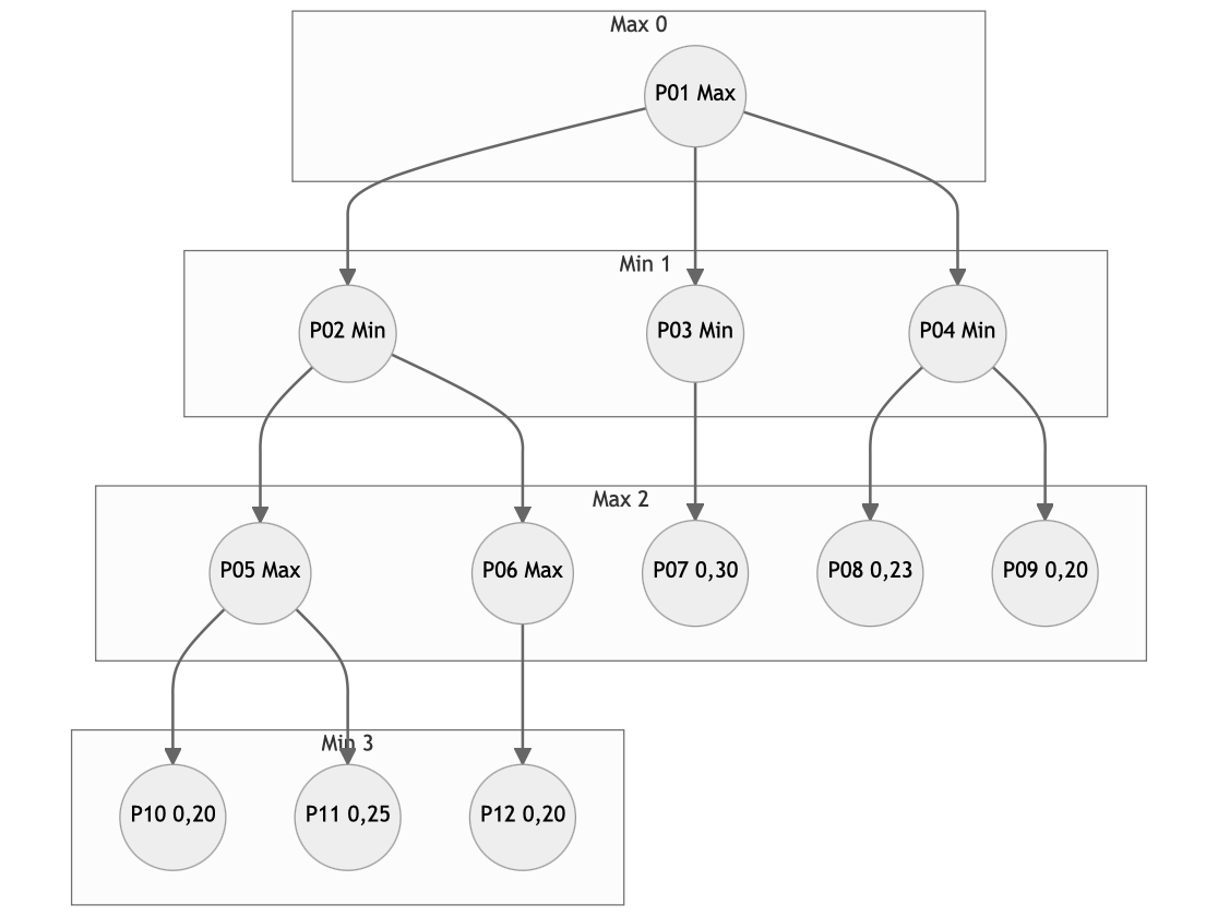
When examining the game tree, it can be noted that not all states are at the same level. For example, state P10 is at the same level as P11 and P12, that is, at level 3. However, P07, P08 and P09 are located at level 2. This disparity in levels implies that it will be necessary to find both the maximum and minimum of those levels respectively.

In practical terms, this means that, in the process of evaluation and move selection, one must search for the maximum possible value at level 3 (where P10, P11 and P12 are located), while at level 2 the minimum value will be sought. These search and selection operations will allow determining the most favorable moves for each player, considering both the possibilities of success and the countermeasures that opponents may adopt at each level of the game tree.

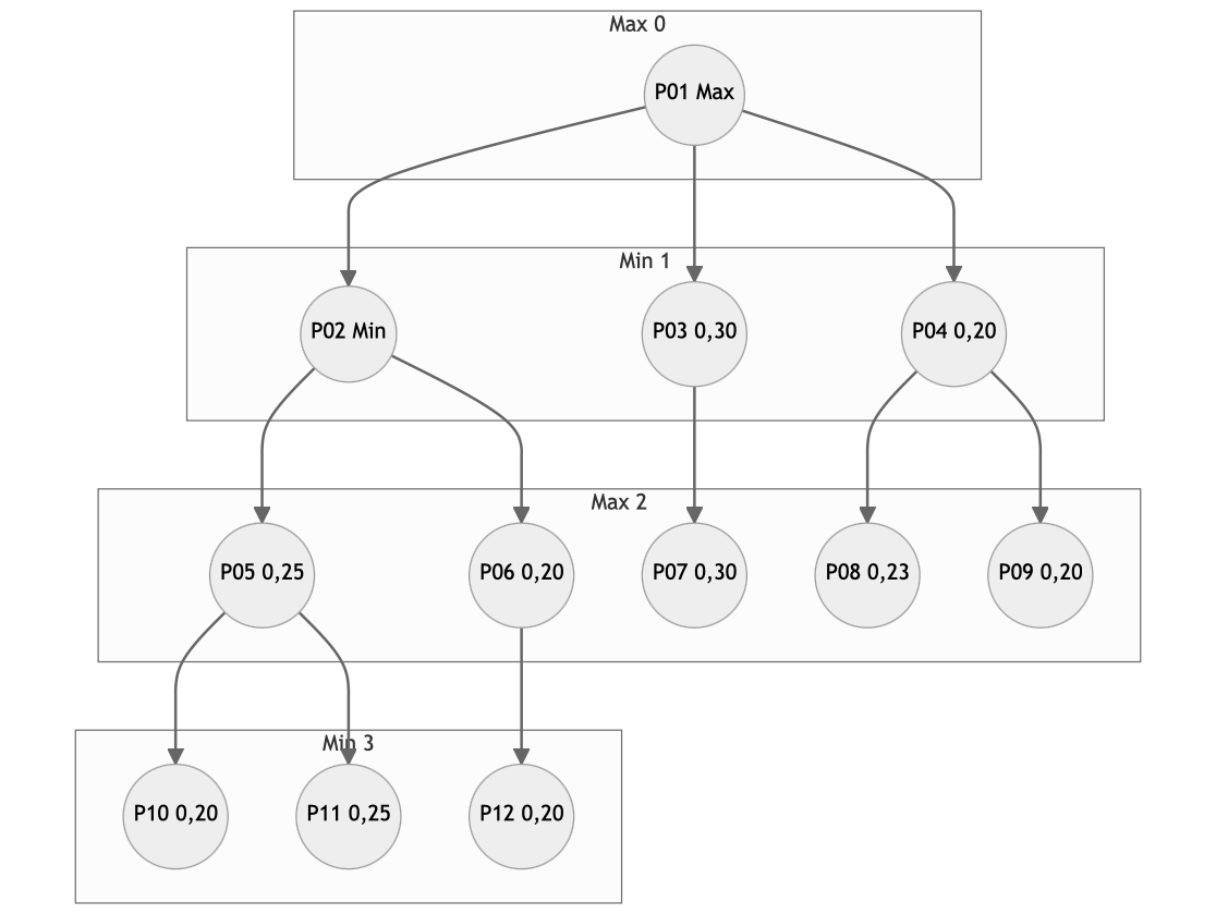
In the second phase of the algorithm, maximization and minimization are performed to calculate the values of some states at level 2 and level 1, respectively.

At level 2, state P05 is calculated as the maximum between the values of P10 and P11, which results in a value of 0,25. On the other hand, state P06 takes the value of P12, since P12 is its only descendant in the game tree.

Regarding the minimization process at level 1, state P03 takes the value of P07, since P07 is its only descendant. On the other hand, state P04 takes the minimum value between P08 and P09, which is 0,20.

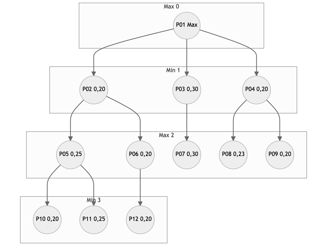
In the third phase of the algorithm, the calculation of the value of the remaining state at level 1, which is P02, is performed. In this case, the value of P02 is determined as the minimum between the values of P05 and P06, since it is at an odd level, which implies a minimization phase.

With this additional calculation, all the necessary values have been obtained to calculate the value of the original state. This original state is represented in the fourth phase of the chess Minimax example. From the values calculated in the previous phases, the optimal value of this state can be determined according to the minimax algorithm, considering the maximization and minimization strategies at the corresponding levels of the game tree.

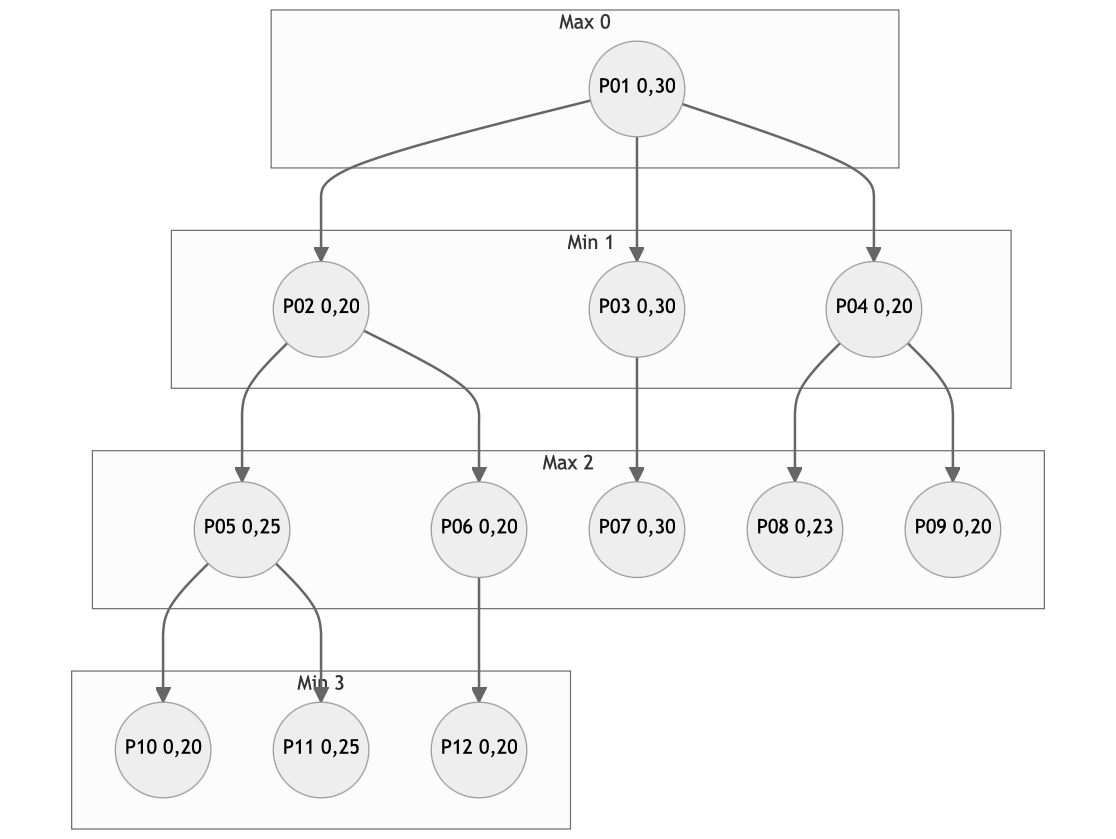
Finally, the value of the initial state, designated P01, is calculated. This calculation is performed by taking the maximum value among states P02, P03 and P04, resulting in a value of 0,30. This value indicates that the descendant state that possesses it corresponds to the best potential move. Thus, according to the developed game tree, the transition to state P03, or what is equivalent, the move Cf3, is identified as the best option.

It is important to emphasize that game trees generated by computers can reach a formidable size, even containing more than one million states, a number that significantly eclipses the number of states in the example provided above. Therefore, it becomes essential to explore methods to reduce the size of this tree. In a previous section, it has been presented how it is possible to prioritize certain states based on their value. However, there is a technique that can significantly reduce the size of the game tree, sometimes even cutting it in half. This technique is known as alpha-beta pruning, and can be considered as an improvement of the Minimax algorithm. This topic will be discussed in greater depth in the following section of this chapter.