The n-queens problem

A millenary problem

To stimulate your curiosity and engagement in this fascinating chapter, allow me to reveal an intriguing incentive: there exists a one million dollar reward for whoever manages to discover a deterministic polynomial algorithm that can solve the problem we are about to describe for any value of $n$. Although the term “polynomial algorithm” may be unknown to some, do not worry, in the coming sections we will address it in detail so that you can understand its meaning and relevance.

Now, to keep the excitement growing, it is time to present you with the problem in question:

“Given a chessboard of dimension $n \times n$ (which means that each row and each column has $n$ squares), a solution to the problem consists of placing $n$ queens in such a way that none of them can attack another”.

To express it more clearly, the objective is to place the queens in such a way that they cannot attack each other. This implies that there can only be one queen in each row, column and diagonal. For those who are not familiar with the rules of chess, an appendix has been included at the end of the book that explains how the different pieces move in this game.

In case you are thinking of accepting this challenge, we inform you that solving this problem is equivalent to proving that P=NP, one of the most important and unresolved questions in computation theory. You can find more information about this prize and the contest rules on the Clay Mathematics Institute websitehttps://www.claymath.org/millennium-problems/p-vs-np-problem (last consulted on 8/9/2022).

To familiarize ourselves with the problem at hand, it is convenient to start with the smallest dimensions, denoted as $n$, of the chessboard.

For $n = 1$, we encounter a board consisting of a single square. In this scenario, we have a single queen to place. Due to the board dimensions, there exists only one possible location for the queen, this being the only viable solution for a board of this size.

When increasing to $n = 2$ or $n = 3$, we encounter an obstacle. In these cases, it is impossible to find a solution. The underlying reason for this statement is that on chessboards of these dimensions, queens cannot be placed in such a way that they do not threaten each other, according to the rules of the game.

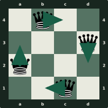
When increasing the board size to $n = 4$, the situation becomes more interesting, as there exist multiple solutions. In particular, there are two possible solutions for a board of this size. One of the solutions can be visualized directly on the board. The other solution can be obtained through a rotation of the board that already has a solution: we simply need to move the queens following the directions indicated by the arrows. In this way, all possible solutions for a chessboard of dimensions $n = 4$ can be explored.

The 4x4 board solutions present both solutions for the eight queens problem on a 4x4 board. The first solution consists of placing the queens on squares a2, b4, c1 and d3. In the second solution, the queens move to the squares indicated by the arrows, being positioned on squares a3, c4, b1 and d2.

In the case of a chessboard of size $n\times n$ with $n = 5$, numerous solutions can be found, with up to 10 possible solutions. However, it must be taken into account that there are really only 2 unique solutions, since the rest are derived from these through reflection and rotation operations.

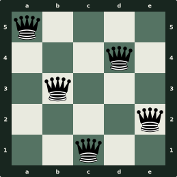
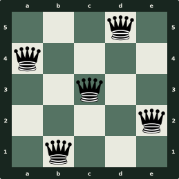
To be more specific, from the first solution (left board), a total of 8 different solutions can be generated, while from the second solution (right board), only 2 distinct solutions can be obtained, applying the rotation and reflection operations mentioned above.

Below, the operation of rotations and reflections is explained in a simple way.

1. Rotation: This operation consists of rotating the chessboard at angles of 90, 180 or 270 degrees clockwise or counterclockwise. When rotating the board, the position of the pieces changes, but the relationship between them is maintained, which can give rise to apparently different but equivalent solutions.
2. Reflection: Reflection involves “mirroring” the chessboard, that is, inverting the positions of the pieces symmetrically with respect to an axis (horizontal, vertical or diagonal). As with rotation, the relationship between the pieces is preserved, so it can also generate solutions equivalent to the originals.

Once the reader has acquired a good understanding of the problem being addressed, it is possible to make some general observations about it. Regardless of the dimension $n$ of the board, there are certain geometric patterns that remain constant and that can help facilitate the search for a solution more effectively. However, in the traditional approach to this problem, it is assumed that some queens are already arranged on the board, which, in most circumstances, hinders the use of the geometric patterns previously mentioned. Therefore, it is imperative to develop an algorithm that can solve the problem under these specific conditions.

One of the geometric patterns considered is that which consists of placing the queens following the movement pattern of the knight in chess, that is, in an “L” shape, to prevent them from attacking each other. However, this solution is only effective in particular cases, since, in most situations, the queens will end up attacking each other. An example of how this pattern works can be seen in the 5x5 board solutions, where all queens are arranged following the knight’s jump. For larger boards, it is possible to use the same technique, but with certain restrictions. The solution shown for an $n \times n$ board is an example of this.

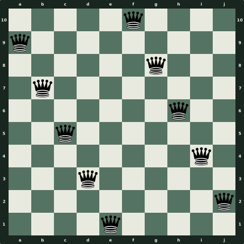
It is essential to note that, although most queens can be placed using the knight’s jump pattern, it is sometimes necessary to dispense with this pattern to satisfy the constraints of the problem.

In summary, although the “L” shaped arrangement strategy can be very useful, it does not constitute a universal solution to solve the problem. In the next section, a universal technique will be presented that will allow the problem to be solved in any situation.

Backtracking versus n-queens

The Backtracking algorithm, also known as “backtracking”, is one of the most widely used algorithmic schemes in solving complex problems. In general, this algorithm allows an exhaustive search in the space of all possible solutions, selecting those that meet the criteria defined by the problem in question. Additionally, its ability to generate all possible solutions allows identifying and selecting the one that is most optimal or favorable, according to the specific requirements of the problem.

Despite these advantages, the use of Backtracking presents a significant disadvantage: the number of possible solutions grows exponentially in most cases. If an attempt is made to generate all possible solutions, the algorithm will have to face the exponential computational cost inherent to this growth.

Fortunately, there are strategies to mitigate this complexity. Two of the most prominent are pruning and intelligent search. Pruning is a technique that allows aborting the exploration of certain branches of the solution space as soon as it is determined that they cannot lead to a valid solution. For its part, intelligent search allows defining the order in which the different branches of the solution space are explored, giving priority to those that, according to a predefined heuristic, are more likely to contain a valid solution. The concept of heuristic, as well as its application in the context of Artificial Intelligence, will be addressed in depth in the chapter dedicated to Artificial Intelligence applied to chess.

Next, we will focus on the application of the Backtracking algorithm to our problem under study.

State representation

When performing a Backtracking through all possible “solutions” or “states”, it is crucial to appropriately define how these states will be represented. For the specific problem we are addressing, which involves the placement of queens on a chessboard, we must also consider that there may be queens that have not yet been placed. So, the question arises: How do we represent this?

An initial idea commonly considered is to represent the position of a queen through its coordinates on the board. Those queens that have not yet been placed are simply not included in the list of coordinates. The board used for the representation shows the board that will be used to show the different representations.

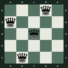
The coordinate representation corresponding to the board presented above is as follows:

$$[\text{a4}, \text{b1}, \text{c3}, \text{d5}]$$

Since there are four queens, there would only be four coordinates in this representation, although it is possible to easily place a fifth queen on the board, adding it at coordinate e2.

The representation we have used so far is useful, but can be improved, especially considering that, according to the rules of the problem, there can only be one queen in each column and row. This restriction allows us to significantly simplify the representation.

The idea is to use a list of integers of size $n$. For each column, we will indicate in the list which row the queen is in. Thus, the first position of the list corresponds to column “a”, the second to column “b”, and so on. If in column “a” the value 3 appears, this indicates that the queen located in column “a” is in row 3. If a queen has not been placed in a particular column, we assign a value of -1 to that position in the list.

Therefore, the new representation of the board in the representation board would be:

$$[4,1,3,5,-1]$$

According to the representation, the queen of the first column is in row 4, the queen of the second column in row 1, the queen of column 3 in row 3, the queen of column 4 in row 5 and the queen of column 5, not yet being placed, has a -1.

Thanks to this representation, an algorithm can be created in a simple way to solve this problem.

Algorithm operation

To illustrate how the Backtracking algorithm operates, a step-by-step example of how a specific case is solved is first presented. Subsequently, a general overview of the algorithm’s operation is provided, representing it through a flowchart.

The initial backtracking configuration shows the initial configuration of the queens that will be used to solve the problem.

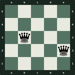
The first step of the algorithm consists of establishing a representation corresponding to the initial board. This representation is obtained as follows:

$$[-1, \ 3,-1,-1, \ 2]$$

The algorithm will proceed column by column, solving those columns whose value is -1, that is, the columns that do not yet have a queen placed. The process begins with column “a”.

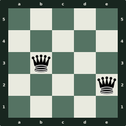
As can be seen, there are two possible rows to place the queen: 1 and 5. The first is chosen, since 1 is less than 5, although the choice could be made in any order. Once the queen is placed in the first column, in row 1, we proceed to the next step, which consists of placing the queen in the third column (the queen in the second column is already placed).

$$[\ 1, \ 3,-1,-1, \ 2]$$

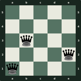
At this point, there is only one viable option, which consists of placing the queen of column “c” in the fifth row, so no branching occurs. A branching occurs when there is a choice between different options to place the queen in a given row.

$$[\ 1, \ 3, \ 5, -1, \ 2]$$

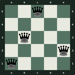
After placing the last queen, we encounter an unpleasant surprise, since there is no square in column “d” that is not being attacked by another queen. Consequently, it is impossible to place a queen in that column without it being attacked. This is when the “backtracking” algorithm comes into play: since a solution could not be found on this path, it is necessary to go back to the previous branching, where one had to choose between different options. In this specific case, we go back to the first column, where one had to choose between rows 1 and 5. If there had been several options in column 3, we would have gone back to that column. Finally, the queen of column “a” is placed in the fifth row.

$$[5, \ 3,-1,-1, \ 2]$$

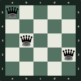
The solution continues with the placement of the next queen in the only position that remains available. This position corresponds to the first row of the third column.

$$[5, \ 3, \ 1 ,-1, \ 2]$$

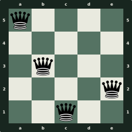
Fortunately, in this case, it is possible to continue placing queens in the next column.

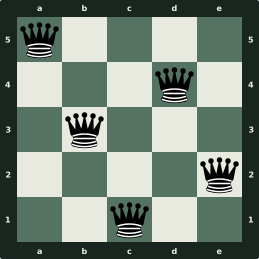
Once a queen has been placed in each column and it has been confirmed that none shares the same row or diagonal with another, we can deduce that we have found a solution. According to the specific needs of the problem, we could stop at this point or continue our search until discovering all possible solutions. In the present case, since there are no more branchings, it is evident that we have arrived at a single solution.

After analyzing the algorithm, a pertinent question arises: How does the computer determine that there are not two queens in the same column, row or diagonal? Regarding the column, we would not have to verify it, since the state representation already ensures it. Regarding rows, it would be simple to check it by examining the current state list and verifying if the row number is already in that list. However, there is an even more efficient method that would involve using a list of 0s and 1s of size equal to the number of rows. In this list, a 0 in position $i$ would indicate that row $i$ is unoccupied, and a 1 would indicate otherwise. This type of value, which can only be 0 or 1, is known in computer science as boolean.

Finally, in the case of diagonals, the situation would be somewhat more complex, but fortunately there is a formula that considerably simplifies this process if we convert the columns into numbers. To carry out this conversion, each letter is simply replaced by its corresponding position in the alphabet: “a” becomes 1, “b” becomes 2, and so on. With this equivalence in hand, we can apply the formula.

Two queens, represented by positions $i$ and $j$ in a vector $V$, are on the same diagonal if and only if $|i - j| = |V[i] - V[j]|$. In other words, the absolute difference between columns $i$ and $j$ must be equal to the absolute difference between rows $V[i]$ and $V[j]$. The absolute value operator, $|\cdot|$, is used to eliminate any negative sign. For example, $|2| = 2$ and $|-3| = 3$.

A disadvantage of this method is its computational complexity, since it requires comparing each queen with all the others. To illustrate, with $n = 8$ queens, $7 + 6 + 5 + 4 + 3 + 2 + 1 = 28$ comparisons would be needed. However, there is a more efficient way to approach this problem: marking the diagonals already occupied to avoid repeating unnecessary comparisons. Another faster method to represent these states would be using bit sets or bitsets [Steven Halim, 2013].

Once an example has been analyzed and its operation understood, we can define the algorithm through a flowchart that illustrates the general resolution process. The N-queens backtracking flowchart shows said flowchart. In a real program, it would be necessary to detail more specifically the actions performed in each step of the flowchart, but since this book has an informative character, it is not necessary to go into those technical details.

Start → Input → Placed? → Can place queen in row? → Solution → End → Backtrack to last branching → Add queen

Below, each of the algorithm steps represented in the flowchart is described in detail.

1. Start: The algorithm is initiated.
2. Input: The problem is introduced with the queens already placed on the board.
3. Placed?: It is verified if all queens have been placed on the board. If the answer is affirmative, the algorithm has found a solution and proceeds to terminate. Otherwise, the algorithm continues with the next step, which consists of determining whether it is possible to place a queen in the next row without interfering with the queens already placed.
4. Can place queen in row?: It is evaluated whether it is possible to place a queen in the current row without it being attacked by other queens present on the board. If the answer is affirmative, the algorithm places a queen in the current row and advances to the next step. If the answer is negative, the algorithm backtracks to the last branching, that is, to the point at which it had to choose between different options to place the queens.
5. Backtrack to last branching: The algorithm returns to the last branching, removing the queen placed at that instance from the input.
6. Add queen: A queen is placed in a valid position of the current row, and then step 3 is returned to verify if all queens are placed on the board.
7. Solution: An output is produced that contains the arrangement of the queens on the board, constituting a solution to the problem.
8. End: The algorithm concludes its execution.

In summary, the Backtracking algorithm applied to the $n$-queens problem is based on exploring possible solutions by placing queens on the board iteratively. If at some point it is not possible to place a queen in the current row, the algorithm backtracks to the last branching and tries with a different arrangement. This process is repeated until finding a solution in which all queens are placed on the board without attacking each other.

Algorithmic complexity

The objective of this chapter is to use the algorithm we have previously discussed as a pretext to introduce the concept of algorithmic complexity. Algorithmic complexity emerges as a tool to measure and compare the efficiency of different algorithms in a way that does not depend on specific computer hardware. To establish this hardware-independent measure, we resort to a theoretical machine: the Turing Machine.

Before moving forward, we will provide a definition of the Turing Machine. Note that, given the informative objective of this book, the rigor of a mathematical definition is not sought.

The Turing Machine, conceived by Alan Turing, consists of an infinite tape in both directions. This tape is analyzed by a read and write “head” that can move left or right. This head is capable of reading and writing various symbols on the tape. The machine has a set of states that, depending on the symbol read, tell it what action to perform.

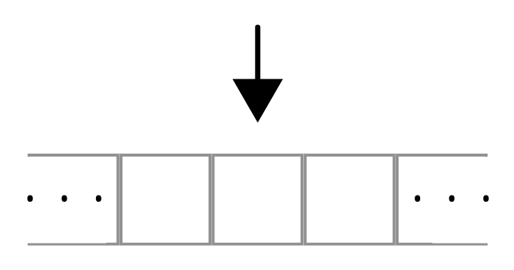
We can offer a more formal definition of the Turing Machine through the following tuple:

$$MT = \{ \sum,Q,q_0,F,\delta \}$$

This tuple consists of five elements: the alphabet, the set of states, the initial state, the final states and the transition function, respectively.

$\sum$ or alphabet: Represents the set of symbols that can be used in a specific Turing Machine. This includes the blank symbol, commonly represented by ”.”.

$Q$ or set of states: These are the states that the machine can adopt. These states, together with the symbols, determine the actions that the head must perform.

$q_0$ or initial state: It is the state in which the Turing Machine begins. It is unique.

$F$ or final states: These are the states that, when reached, allow the machine to terminate its process. There can be several.

$\delta$ or transition function: It is a function that, given an input consisting of the current state and the symbol read by the head, returns the next state to which the machine must transition, the symbol that the head must write in its current position and the direction in which the head must move.

Although the Turing Machine is a valuable tool for understanding computation theory, its abstract nature means that it is rarely used in practice to determine the complexity of an algorithm.

That said, the Turing Machine possesses impressive computational power and is capable of solving a vast number of problems. However, there are certain problems that are beyond its capabilities, often associated with the so-called halting problem. These problems are intrinsically unsolvable, not only for the Turing Machine, but for any modern computer, given that all computers are based on the structure of the Turing Machine.For more information on this aspect of computation: [Noson S. Yanofsky, 2016]

In practice, to calculate the complexity of an algorithm, we use a series of well-established principles and methods. We begin by defining a function that represents the approximate complexity of the algorithm. This function takes as its value a variable that represents some key aspect of the algorithm’s input.

For example, in the $n$-queens problem, this representative variable is $n$, which indicates the size of the board. In a version of the problem in which some queens have already been placed, it would be more appropriate to use $n$ minus the number of queens placed; therefore, the most suitable variable in this case would be the number of queens remaining to be placed. If the algorithm must operate on a list or a vector, this representative variable is usually the size of these.

To determine the output value of the complexity function, we must analyze how many times a given representative operation is executed as a function of the chosen variable. In the case of the $n$-queens problem, the representative operation would be the number of times a queen is placed on the board, which at a lower level translates into an assignment in the column list.

In most cases, it is impossible to determine precisely the exact number of times a particular operation will be executed. In such cases, it is useful to consider the worst possible scenario. In this way, we can obtain an upper bound for complexity, which means that, for a given input, the algorithm will not take more time than the time corresponding to the worst case.

Even so, it will often be impossible to find an exact measure of complexity. However, what interests us is not so much the accuracy of the measure, but the way in which the number of operations grows as a function of the representative variable of the input. This growth is grouped into different categories or “families” of functions, according to their growth rate. This concept is known as big-$O$ notation.

The most common families, ordered from best to worst in terms of growth, are as follows (we will use $n$ to represent the representative variable):

$O(1)$: Regardless of the value of $n$, the execution time of the algorithm remains constant. This is the type of complexity associated with the basic operations (additions, subtractions, multiplications, etc.) that a computer can perform, such as adding two numbers or performing assignments.

$O(\log n)$: This is a very favorable growth rate, as it is inversely proportional to exponential growth. Examples of algorithms that exhibit this type of growth are binary search and search in a binary search tree.

$O(n)$: In this case, the execution time of the algorithm grows linearly with $n$. Although it is slower than $O(\log n)$, it is still acceptable for most applications. Examples of this type of growth are searching for an element in an unsorted list or vector and raising a number to a power.

$O(n \log n)$: This type of growth is slightly faster than $O(n)$, and is common in algorithms related to sorting elements. Examples of algorithms with this type of growth are Heapsort and Quicksort (in the average case).

$O(n^a)$ where $a > 1$: This type of growth includes all algorithms whose execution time grows as a polynomial of $n$, with the exception of the linear cases already mentioned. Although the value of $a$ can be high, this type of growth is still preferable to the growth types we will mention next. Examples of this type of growth are matrix multiplication $O(n^3)$ and algorithms that use two nested loops $O(n^2)$.

$O(a^n)$ where $a > 1$: This is the beginning of algorithms with non-polynomial execution time, and they are the nightmare of any programmer. Even if $n$ is small, the computation required to solve the problem can be immense. Examples of problems with this type of growth are boolean satisfiability and partitioning a set into two subsets of equal sum.

$O(n!)$, $O(n^n)$: These are the fastest growth cases and are among the most difficult to handle. When $n$ is a large number, both $n!$ and $n^n$ grow faster than any exponential, regardless of the value of $a$ in the exponential. Examples of problems with this type of growth are the $n$-queens problem and the traveling salesman problem.

Once the families are defined, we can use some simple practical rules to calculate the complexity of a specific problem. First, we define basic operations, which are the different arithmetic, logical, assignment and similar operations. All these operations have a complexity $O(1)$, that is, they are constant, and constitute the most basic building blocks of any algorithm.

Linear complexity appears when one or more of the basic operations defined above are executed in a loop that iterates a number of times that grows linearly with $n$. For example, if the value 1 is assigned to all elements of a list of size $n$, the complexity will be $O(n)$. To achieve a complexity of $O(n^2)$, you need to have a nested loop structure in which both loops are iterating proportionally to $n$. A common example of this is when all pairs of elements in a list are traversed. In general, if you have $a$ nested loops that iterate proportionally to $n$, you will get a complexity of $O(n^a)$.

On the other hand, $O(\log n)$ complexity is often achieved through a “divide and conquer” approach, in which the problem is divided into successive halves until reaching a base case. Binary search is a common example of this.

For exponential complexities $O(a^n)$, they often arise in algorithms that explore all possible combinations or permutations of a set. The traveling salesman problem is a notorious example.

Finally, calculating the complexity of an algorithm can involve adding the complexities of the different parts of the algorithm. However, when adding complexities, only the fastest growing one is relevant. For example, if one part of your algorithm has a complexity of $O(n^2)$ and another part has a complexity of $O(n)$, the total complexity will be $O(n^2)$, since $n^2$ grows faster than $n$. This principle applies to all forms of combining complexities.

It is important to remember that these are general rules and that there may be cases in which these rules do not apply exactly. However, they are a good guide to understanding how an algorithm scales as the input size increases. Once these concepts are known, we can begin to analyze the complexity of the $n$-queens.

In exploring the $n$-queens problem, we have considered various strategies for its solution, based on different state representations. Likewise, we will analyze the complexity of these solutions following the same criterion.

Consider a 4x4 board on which we need to place 4 queens. If we generate all possible combinations regardless of order, the calculation would be as follows:

$$\frac{16!}{4!(16-4)!} = \frac{16 \times 15 \times 14 \times 13}{4!} = 1820$$

To arrive at this result, we reason as follows: there are 16 squares available for the first queen, 15 for the second, 14 for the third and 13 for the last. Since order does not matter, we must divide by $4!$, according to combinatorial principles. This result can be generalized for an n x n board with the following formula:

$$\alpha(n) = \frac{(n^2)!}{n!(n^2-n)!} = \frac{n^2*(n^2-1)* ... * (n^2-n+1)}{n!}$$

Thus, $\alpha(n)$ indicates the number of ways to place $n$ queens on an n x n board.

In previous sections, more efficient representations of a solution were discussed rather than simply using coordinates. For example, we could assign a number between $1$ and $n$ (both inclusive) to each column, which represents the row in which the queen of that column is placed. This representation would significantly reduce the number of possible options.

For a 4x4 board on which we must place 4 queens, each column offers four options, which is repeated four times. This number is considerably high for a 4x4 board. The general formula in this case would simply be:

$$\alpha(n) = n^n$$

These two methods present some of the worst complexities we have analyzed so far.

If we remember, the search can be optimized by discarding some possible solutions as they are generated. For example, it is evident that any configuration that places two queens in the same row is not a valid solution, so it can be discarded immediately and avoid wasting unnecessary resources. However, calculating complexity in this case is a challenge, as we need an approximation; it would be impossible to find a formula that provides the exact complexity for any $n$.

We can discard the rows in which we have already placed a queen, reducing in each step the number of rows to check in the next column. For diagonals, the situation is more complicated. In the worst case, we can discard one square in the next column, but we may not be able to discard any in subsequent columns. In the worst case, therefore, the formula for this method would simply be the factorial of $n$. In the first column, there are $n$ options; in the second, $n-1$; and so on. The formula would therefore be the famous factorial.

$$\beta(n) = n!$$

This is the standard performance of the backtracking algorithm for the $n$-queens. Results can be further improved using heuristics or more efficient representations of diagonals, but this is beyond the scope of this book.

In conclusion, after having analyzed the complexity of the $n$-queens problem, we can affirm that no algorithm has yet been found capable of solving it in a reasonable time for large values of $n$. That is, no deterministic polynomial algorithm has been discovered that solves it. Therefore, it is classified as an NP-hard problem.

In general, problems can be divided into two types according to their difficulty: easy, if they can be solved in deterministic polynomial time; or difficult, if a deterministic polynomial algorithm that solves them cannot be found. The great unsolved question is whether both sets are identical and, therefore, there exists a deterministic polynomial algorithm to solve any computable problem. That is precisely the question

The amazing exponential growth

Exponential growth is often portrayed as a devastating and uncontrollable force. But is it really that bad? To appreciate the dizzying speed with which an exponential function can grow, let us turn to the ancient legend of the origin of chess.

According to the narrative, a monarch of a distant kingdom, overwhelmed by boredom, convened a contest in which his subjects could present a game for his entertainment. The creator of the game that most delighted the king would receive any reward he desired. Among the numerous proposals, one stood out above the rest: chess. The inventor of the game, a man of humble condition, asked the king to place one grain of rice on the first square of the chessboard, two grains on the second, four on the third, and so on, until reaching the sixty-fourth square.

The king, initially, laughed at the modest request, but when his counselors calculated the amount of rice needed, they were astonished. There was not enough rice in the entire kingdom, not even in several generations, to fulfill the inventor’s request. When the king understood the magnitude of the request, he could only admire the cunning of the humble creator of chess.

After hearing this story, it is natural to wonder how many grains of rice would be required. To answer this question, we first consider how many grains are in each square. In the first square there is one grain, that is, $2^0$, in the second there are two grains or $2^1$ and in the third there are $2^2$ or four grains. Continuing with this pattern, the total amount of grains can be calculated mathematically using a summation (allows adding a series of numbers that follow a pattern):

$$\sum_{k=0}^{63}{2^k} = 2^{64} - 1 = 18446744073709551615 \textrm{ grains}$$

The formula on the left sums all the grains from each square, the one in the center uses a “trick” to simplify the sum with exponentials, and on the right the total number of grains needed is shown. The figure is astonishing. To put it in perspective, current world rice production is approximately 743 million tons, and each ton can contain about 50 million grains. Therefore, the total world production would be about 37150 trillion grains.

Comparing this figure with the number of grains required for the chessboard, it would take almost 500 years of production to meet the demand, as shown in the following calculation:

$$\frac{18446744073709551615}{37150 * 10^{12}} = 496.55 \textrm{ years}$$

Thus, as can be seen, exponential growth is truly fast and can become overwhelming, as has been exposed in the previous sections of this chapter. Therefore, it is crucial not to underestimate its impact.

The enigma of P=NP?

The P=NP? problem seeks to determine whether the set P, referring to algorithms that can be solved in deterministic polynomial time, is equivalent to the set NP, which comprises algorithms solved in non-deterministic polynomial time. An important observation to keep in mind is that P is a subset of NP, since deterministic algorithms are included in the non-deterministic category. That is, a P algorithm will also be NP, but an NP algorithm will not necessarily belong to P. Within NP there exists a subset called NP-complete problems for which, to date, an algorithm belonging to P has not been found. The search for a solution to the P=NP? problem focuses on demonstrating that there exists a P algorithm for these problems.

From a theoretical point of view based on the Turing Machine, the problem can be defined as follows:

“P=NP if there exists a deterministic Turing Machine with a polynomial time upper bound that can transform a non-deterministic Turing Machine with polynomial time upper bound into a deterministic Turing Machine with the same upper bound.”

This statement can be complex at first. In the case of non-deterministic Turing machines, a particular state and the reading of a symbol can trigger one or more actions instead of a single one, as happens with deterministic machines. This characteristic, applied to computers, implies that different actions must be executed, without knowing which of them will lead to the solution, causing the dreaded exponential complexity.

In summary, solving the P=NP problem would consist of finding a deterministic polynomial algorithm that can transform any non-deterministic polynomial algorithm into a polynomial one, or demonstrating that such an algorithm does not exist. Either of these solutions would grant the discoverer a one million dollar prize.

To simplify, it has been shown that there exists a non-polynomial problem, boolean satisfiability, to which any polynomial algorithm can be converted. This problem consists of determining whether, given a logical expression, there exists an input that makes the formula true. The proof of this fact exceeds the scope of this book, but an intuition of why this might be so is related to the fact that computers are, ultimately, a series of logic gates. This was the first problem discovered of the so-called NP-complete problems, to which all other NP problems can be converted through a polynomial algorithm.

NP-complete problems are quite common in everyday life, and many of them are related to graphs, which will be discussed in the next section. They are also frequently found in optimization problems, among others.

It is important to mention that, in practice, approximate algorithms are usually used to solve these types of problems, with the objective of eluding exponential complexity. These algorithms allow finding a solution that, although not optimal, can be valid according to the defined criteria. In other words, if an exponential algorithm is used for small inputs, it might be possible to find the best solution. However, in the case of very large inputs, an approximate algorithm will be used, which sometimes will not provide the best answer.