The knight's tour

The Jumping Knight

In this section, we will delve into the exploration of one of the most intriguing problems originating from the fascinating world of chess. The protagonist of this enigma is the knight, a piece whose singular type of movement distinguishes it from all other pieces on the chessboard. This peculiarity makes this problem a challenging intellectual pastime. Without further ado, the definition of the problem:

“We place the knight on an initial square on a board of dimensions $m \times n$. The objective is to find a path that visits each square of the board exactly once.”

In simpler terms, the challenge consists of traversing all squares of the board, without repeating any, using the characteristic “L” movement of the knight. When facing this challenge for the first time, one is likely to realize that it is not trivial at all, and it may require several attempts to achieve it even on the classic $8 \times 8$ board. It is important to note that the board does not necessarily have to be square; it can be any rectangle.

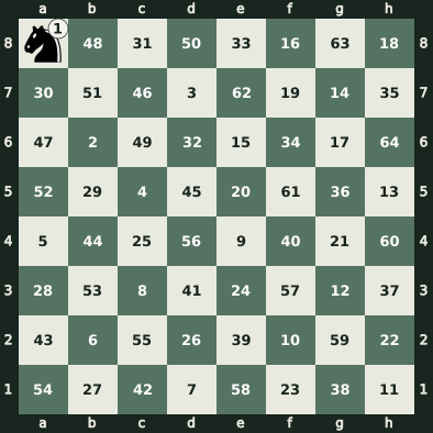
This problem has captured the attention of notable mathematicians throughout history. Among them stands out Leonhard Euler, considered one of the most preeminent mathematicians of all time. Euler not only managed to solve this problem for an $8 \times 8$ board, but he also constructed a semi-magic square in which each row and column sums to 260, the halves of the rows and columns sum to 130, and each number represents the order of the movement with which the knight visited that particular square.

The elegance of this solution can be appreciated in the Euler magic square.

Beyond this intriguing construction, this problem can also be used as a means to generate computational art. Below is a series of artistic compositions inspired by the movements of a knight:

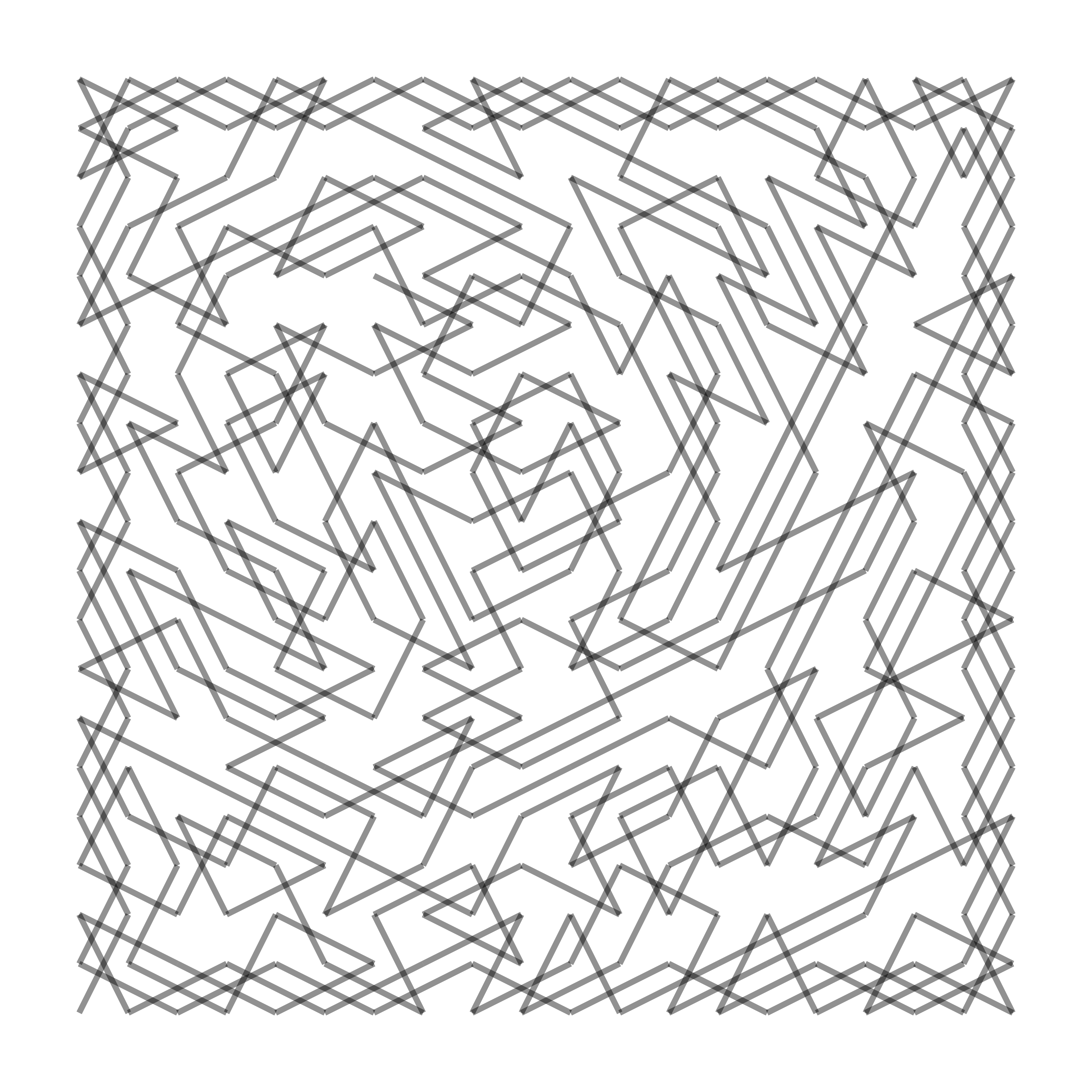
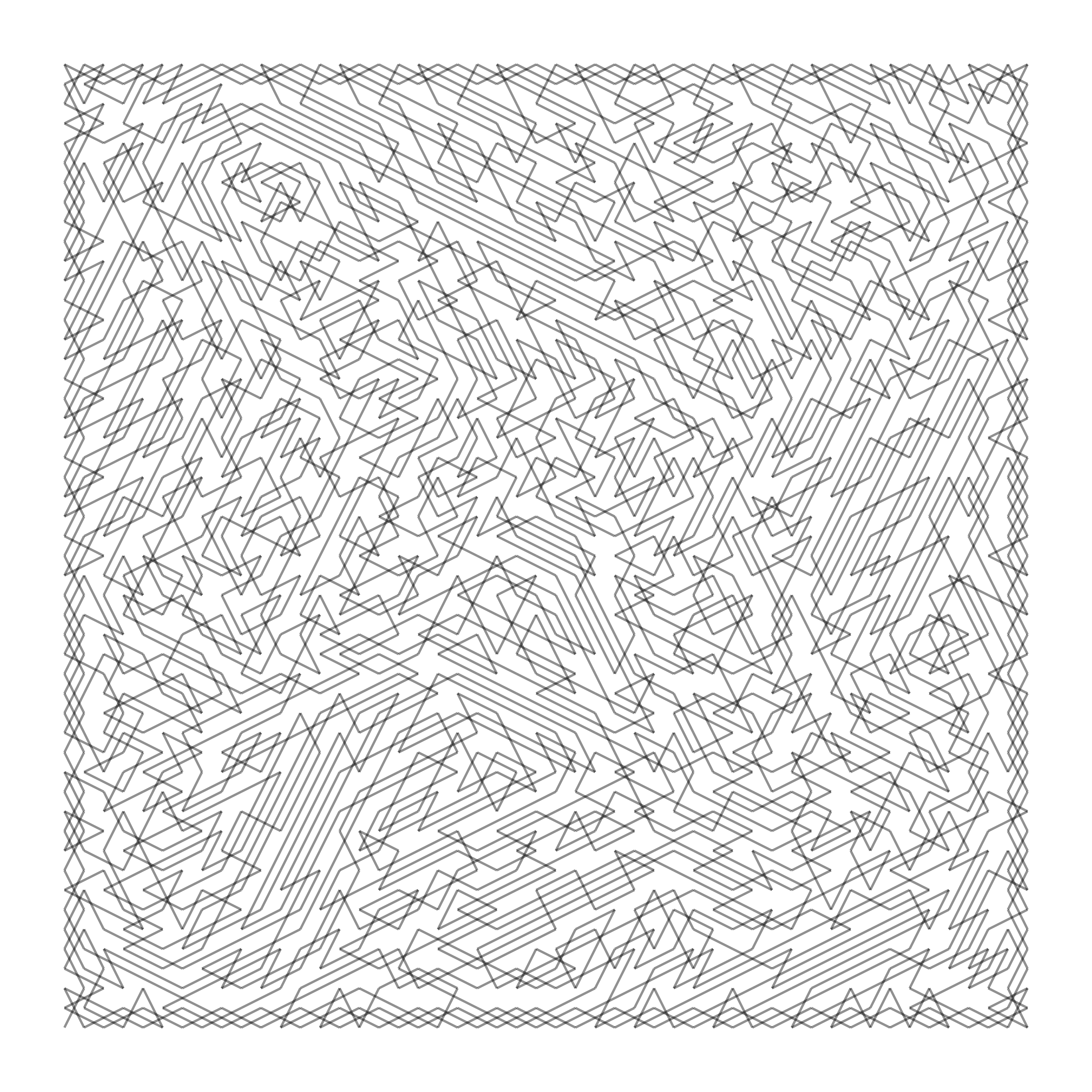
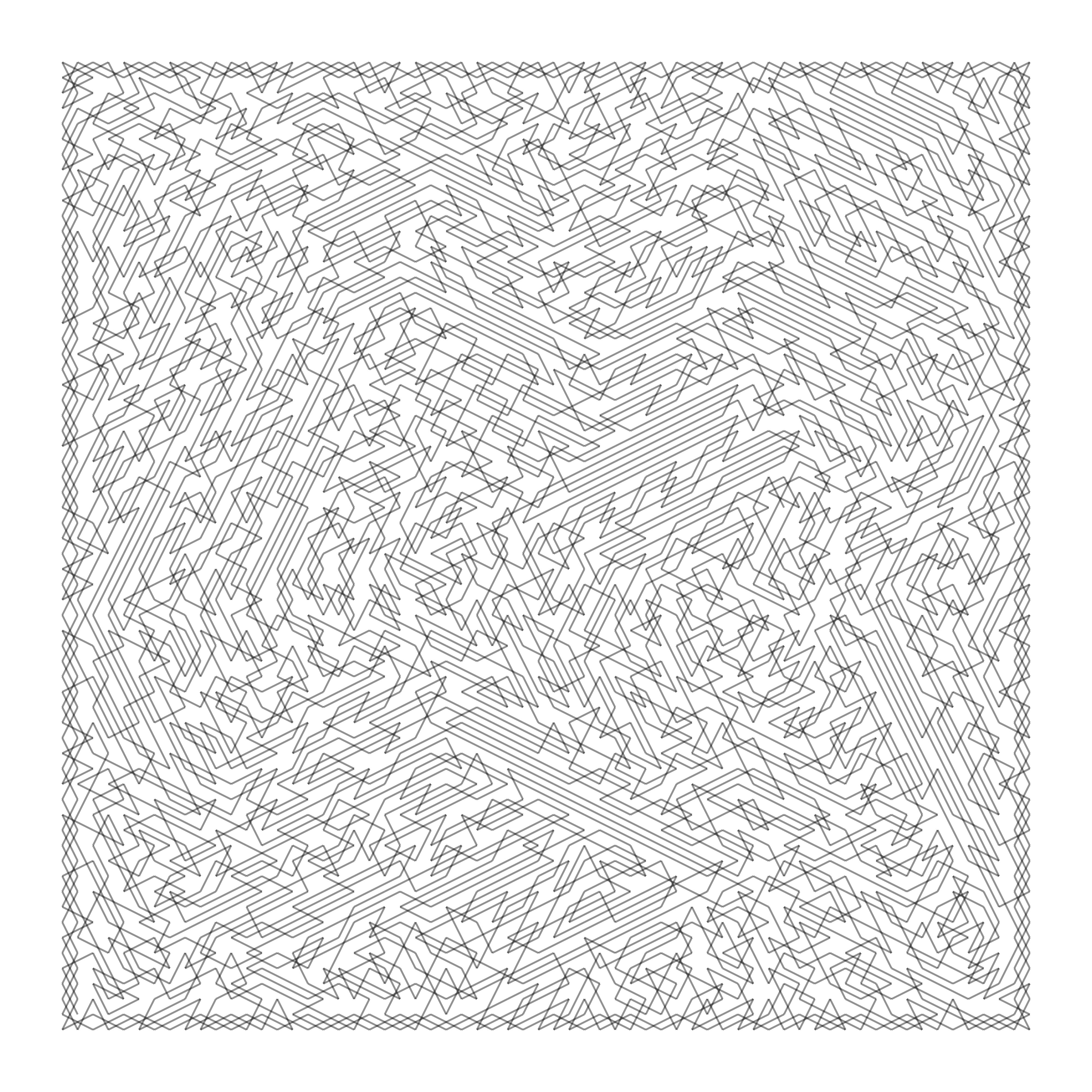
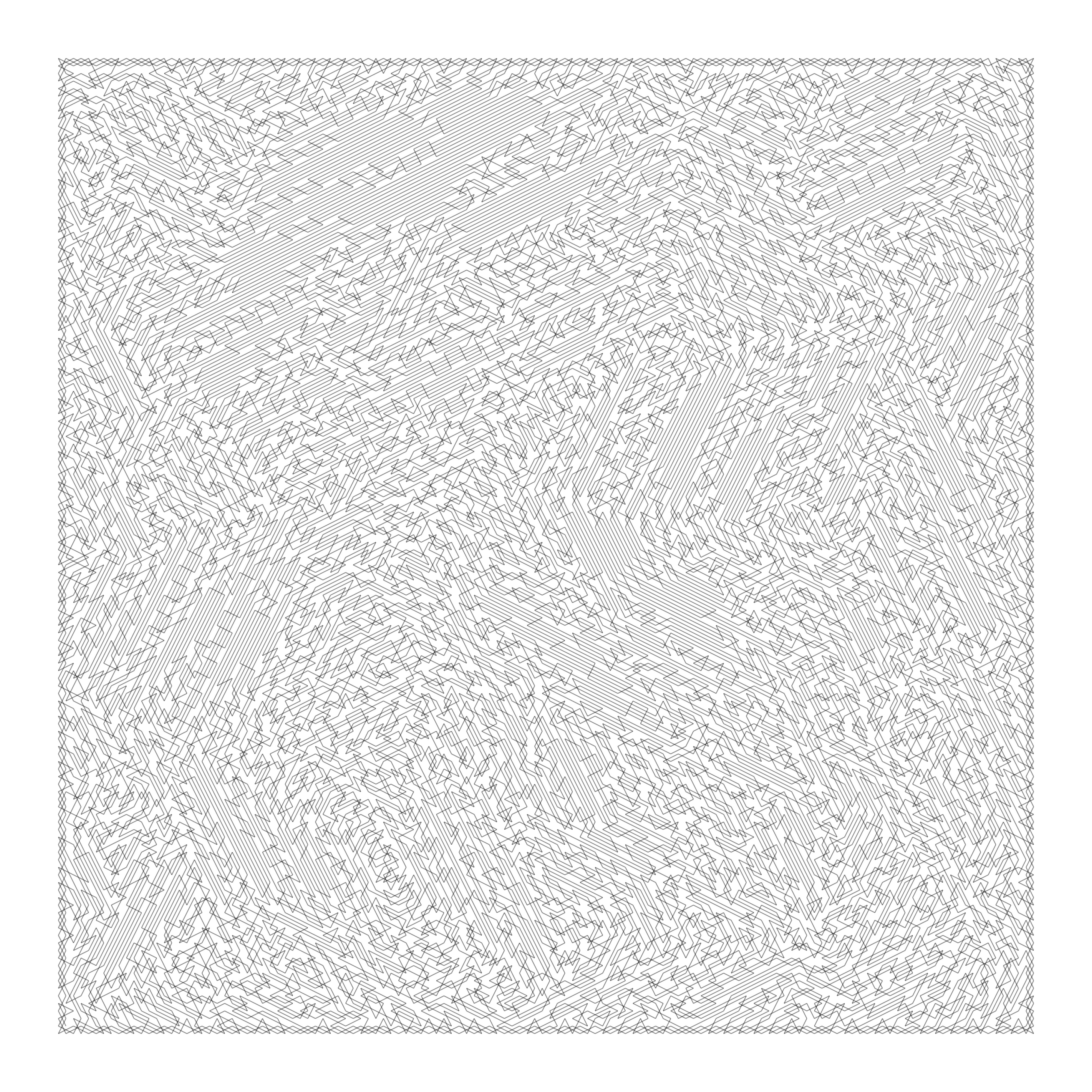
The works represented correspond to boards of different sizes: 20x20 (top left corner), 50x50 (top right corner), 64x64 (bottom left corner) and 130x130 (bottom right corner). Each of these compositions illustrates the rich variety of patterns that can emerge from the simple but challenging task of traversing a chessboard with a knight.

To further relate the reader to the problem, I will proceed to show the solution of an 8x8 board using arrows:

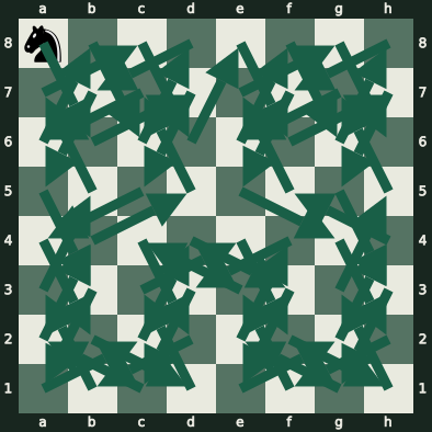
A crucial observation in solving this problem is that the first squares the knight visits tend to be located in the regions furthest from the center. This technique plays a fundamental role in solving the challenge posed. In case you haven’t realized, it is the solution to Euler’s magic square shown above.

The knight’s tour in this context is closely linked to one of the most relevant problems in the field of computer science: the known problem of finding a Hamiltonian path, which is classified as an NP problem.

Hamiltonian paths and graphs

The Hamiltonian path problem is defined as follows:

“Given a graph, we seek to find a path that visits each of the vertices exactly once”. (A path is the sequence in which the vertices of the graph are traversed).

This definition presents a notable similarity with the concept of the knight’s tour. But what exactly are a graph and its vertices?

A graph is a data structure that provides great flexibility for representing relationships between different elements. It consists of a set of vertices (also known as nodes) and edges (or connections). Vertices can be any type of object, from numbers to words and more complex objects. Edges, on the other hand, connect two vertices if some relationship exists between them. In the case where edges have a numerical value representing some aspect of the relationship between the connected elements, it is called a weighted graph.

Returning to the theme of the Hamiltonian path, by slightly modifying the problem’s conditions, two additional interesting problems arise. If we add the restriction that, upon reaching the last vertex, one must return to the initial vertex, we obtain what is known as a Hamiltonian cycle. On the other hand, if we use a weighted graph (each edge has an associated number expressing the cost of using that edge) and we seek the path that minimizes the sum of the values of the traversed edges, we face the traveling salesman problem.

But how do graphs and the different Hamiltonian problems relate to the knight’s tour?

Although it may not be evident at first glance, the chessboard can be considered as an implicit graph, where the vertices and edges are present in a disguised manner. In this case, the vertices would represent the squares of the board, while the edges would model the relationship between two squares. Therefore, there would be an edge between two specific squares if it is possible to move from one to the other through a single knight’s move. Below is an example of a $3 \times 3$ board and its corresponding transformation into a graph that illustrates the previous concept.

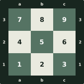
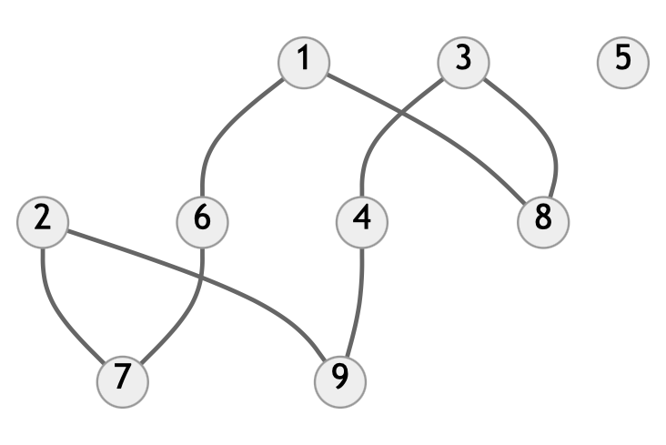
First, the squares of the board are numbered, assigning each of them a natural number (this is a very common technique when working with graphs) and the graph is drawn.

In this representation, it holds that an edge exists between two squares if it is possible to move between them in a single move. For example, from square 9 one can reach squares 4 and 2 through a knight’s move, while square 5 has no edge, since it is not possible to reach it from any other square.

Now then, how is a computer capable of understanding a graph and how is it represented so that it is understood by a machine?

Representation of graphs

The representation of a graph is a crucial element in the efficacy and efficiency of the algorithms that use them. There are multiple representations, each with its unique advantages and disadvantages. Before delving into the explanation of these representations, it is essential to recognize that graphs can be of two types: directed and undirected.

In directed graphs, the edges function as “arrows”, that is, the relationship exists only from one vertex toward another, and it may be the case that a relationship in the opposite direction does not exist. In contrast, in undirected graphs, the edges indicate that a bidirectional relationship exists between the two vertices, as was illustrated with the graph we discussed previously.

Among the various graph representations, the adjacency matrix is a notable option. As its name suggests, it is a matrix in which row $i$ and column $j$ represent the relationship from vertex $i$ toward vertex $j$.

If we are working with an unweighted graph, it is common to use a 1 to denote the existence of an edge from $i$ to $j$, and a 0 otherwise. However, if the graph is weighted, we will place the value of the edge connecting vertices $i$ and $j$ in the respective position of the matrix. If no such connection exists, a very large number is often used to indicate that the edge is unusable, although other alternatives also exist.

Take, for example, the adjacency matrix of the graph of a 3x3 board, which would be represented as follows:

It is relevant to note that the adjacency matrix is symmetric. That is, if we swap rows for columns, we obtain the same matrix. This characteristic is always present in the adjacency matrices of undirected graphs, due to the bidirectional nature of their relationships. It may seem that a redundancy of information exists, and indeed, it does. Therefore, we really only need half of the matrix, specifically, the section above or below the diagonal that extends from the top left corner to the bottom right corner, to have all the necessary graph data. Additionally, it is important to point out that both the column and row of 5 are empty, since it is impossible to reach that square or depart from it toward another.

The main advantage of this representation is that it allows querying in constant time whether one can pass from one vertex to another. This is particularly useful in the implementation of two widely used algorithms in graphs: Warshall and Floyd. Warshall is useful for determining if a path exists between a vertex and any other, and also provides said path. On the other hand, Floyd operates on weighted graphs and provides the shortest path between two vertices, if it exists, and the value of said path.

However, the adjacency matrix also stores non-existent relationships, that is, the 0s in the matrix. Moreover, these 0s outnumber the 1s, indicating that the number of relationships is small compared to the total possible relationships. This leads us to ask: shouldn’t there be a way to store only the existing relationships in the graph and avoid storing the 0s?

Indeed, the answer is affirmative. For this purpose, the adjacency list can be used. Its main premise is to store only the relationships between the different vertices, which allows for significant memory savings and even, on occasion, computation time. In an adjacency list, each vertex is assigned a list containing the vertices with which it is related. The adjacency list for the previous graph would be presented as follows:

As you can see, a significant reduction in the amount of information stored has been achieved using the adjacency list. In this specific case of the chessboard, we are fortunate as a knight piece can only move to a maximum of two squares. However, as the size of the board increases, the memory efficiency of the adjacency list over the adjacency matrix also increases. This is because, at most, a knight can move to 8 different squares from a specific square, so the list will have at most that number of elements.

The main disadvantage of this method of representation is that, if we need to verify the existence of an edge between two vertices, we must search the list of the first vertex to see if the second vertex appears or not. It is important to mention that this representation can also be used for weighted graphs. In that case, the elements of the lists are replaced by tuples of two values: the vertex and the weight of the edge. This representation may not be suitable for algorithms like Floyd or Warshall The Floyd algorithm finds the shortest path between all pairs of nodes in a graph. On the other hand, the Warshall algorithm determines if a path exists between all pairs of nodes., but it is more efficient for algorithms searching for Hamiltonian paths or cycles.

Finally, it is worth mentioning that another way to represent a graph exists, called an edge list. As its name indicates, this list contains all the edges, each expressed as a tuple of two integers, where the first integer represents the source vertex and the second the destination vertex. However, this method of representation is rarely used.

Having examined the different ways of representing a graph, we are ready to address the Hamiltonian path problem. To solve this challenge, we must resort to a well-known strategy: backtracking.

Backtracking vs. the knight’s tour

Just as in the $n$-queens problem, we face a question: how can we predict if a decision we make will lead us inexorably to a dead end or a valid solution?

We will need the ability to go back and explore other paths to find a valid solution, if one exists. For this reason, backtracking seems the most appropriate option intuitively. However, as mentioned previously, we are dealing with an NP problem. Fortunately, the “knight’s tour” is a specific version of the problem where we can notably improve the efficiency of the algorithm using a heuristic A heuristic is a rule of thumb or approximate method that helps simplify and solve problems, often allowing for finding sufficiently good solutions although not always optimal. known as Warnsdorff’s rule. This rule reduces the complexity of the algorithm, allowing for a solution in linear time.

A heuristic is a guide that orients us toward the states that are more likely to lead to a valid solution. Warnsdorff’s rule advises us to head toward the vertex of lowest degree. Here a new question arises: what is the degree of a vertex?

The degree of a vertex is defined as the number of vertices that can be reached from said vertex with a single move. It is similar to the number of edges of a vertex, but edges leading to an already visited vertex are not counted. If the degree of a vertex is 0, it means that we will not be able to perform any more moves once we reach that vertex. Therefore, we should only head to a vertex of degree 0 if this is the last move we intend to make.

Once we have clarified this term, we can proceed to solve the problem on a 5x5 board. Suppose the initial square of the knight corresponds to a1, that is, a knight situated in the bottom left corner. We will use a matrix of the same dimensions as the board to record the squares we have already visited and advance in the resolution of the problem. This matrix will be of integers, and the value of a square will be the order number in which it was visited. To start, all values of the matrix will be 0, except the initial square, which will have the value 1. Zero indicates that that square has not been visited yet.

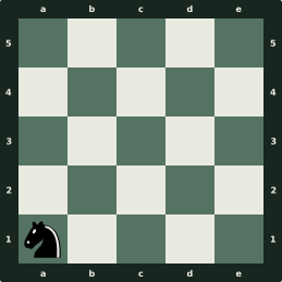
In the first circuit around the board, the knight has passed through the four corners, since these always have degree 1, as they lead to only two squares and one of them will already have been visited (the one through which it reached the corner). In the second move, when moving from square b3 to a5, the rule is clearly applied by preferring to go to corner a5 with degree 1 instead of going to squares c5 or d4 with degree 3. The visited matrix would be as follows, next to the board indicating the knight’s moves:

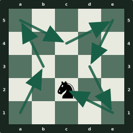
Following the same heuristic, the knight performs a second circuit through the board, obtaining the following board and state:

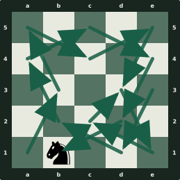
In the last circuit, the board would be completed and the following final board and state would be obtained:

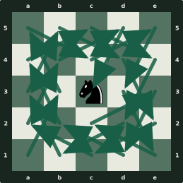
As an interesting result, it is observed that the last square visited is exactly the central one, which in the 5x5 board is the only square with degree 8 at the start of the problem. This demonstrates that the knight, following the heuristic used, manages to reach and visit all the squares of the board, ending in the only square with degree 8 at the beginning.

To conclude, below is the flowchart indicating the operation of the algorithm used to solve the knight’s tour.

Below, each of the algorithm steps represented in the flowchart is described in detail.

1. Start: The algorithm is initiated.
2. Input: The problem is introduced with the initial square of the knight and the size of the board. As the problem progresses, it will include the squares already traversed and the current position of the knight.
3. All squares traversed?: It is verified if all the squares have been traversed with the knight. If so, it terminates and otherwise the algorithm continues in the next phase.
4. Can the knight move to a square?: An attempt is made to place the knight in one of the squares within its reach in a single move. Those squares must also not have been visited. In the event that there is more than one, they are ordered following Warnsdorff’s rule from lowest to highest.
5. Backtrack to last branching: The algorithm returns to the last branching, removing the knight’s last move along with the indication that that square has been visited.
6. Move knight: The knight is moved to the selected square. The square where the knight was previously is marked as visited.
7. Solution: A matrix of the same size as the board used that indicates in which move the knight has visited that output.
8. End: The algorithm concludes its execution.

It can be seen that it is very similar to the $n$-queens algorithm. And it is natural when both use backtracking. The only noteworthy differences are the representation (which is after all the most important part of the algorithm) and the use of Warnsdorff’s rule. The rule simply changes the order in which squares are visited, prioritizing those that have fewer moves available.

Algorithmic complexity of the knight’s tour

In the study of algorithmic complexity, it is usual to take into consideration the worst case, that in which all possible circumstances that can be adverse indeed occur. A simplified strategy to calculate this worst-case scenario could consist of assuming that the knight will always be able to move to the maximum number of squares.

For example, starting from a square on a chessboard, it is possible to perform up to 8 different moves, that is, each vertex in this context has a maximum of 8 edges. This implies that for each square traversed, there are 8 possible choices. Since the board is of dimensions n x m, this decision would be made n*m times, providing the following formula for the worst-case complexity:

Where $n$ denotes the number of rows and $m$ the number of columns. Although this calculation shows exponential growth, fortunately this upper limit is quite far from the true complexity of the problem at hand.

In most cases, the number of choices will be less than 8, given that it may happen that the square under study has fewer than 8 edges, or that some of these edges lead to a previously visited square, which will not need to be considered again. Applying Warnsdorff’s heuristic, the traversal of the board is performed from the outside toward the inside, which implies that, upon reaching the central squares, the squares peripheral to these will already have been visited, thus avoiding considering numerous trajectories.

With these considerations, the problem can be solved in a reasonable time through a computer, even when $n$ and $m$ are greater than 100. In the event that the knight’s tour seeks to find a Hamiltonian cycle, that is, a traversal that from the last square allows returning to the initial one in a single move, this heuristic would not reduce the complexity so significantly, as it does not orient the search toward the appropriate last square.

Comparing the complexity of the general Hamiltonian path/cycle problem and the traveling salesman problem, a notable difference can be observed regarding the knight’s tour, given that each vertex in these problems could have an indeterminate number of edges, from a single one to an edge directed to each of the other vertices.

Again, for the complexity calculation it is necessary to consider the worst case, in which all vertices are connected to all others. If we consider a graph with $n$ vertices, where an edge exists between all vertices, in the first vertex we would have to choose between $n - 1$ edges, since only this first vertex has been visited. In the second vertex, we would have $n - 2$ edge options, since the first vertex and the current one have already been visited. Continuing with this procedure, one can see its similarity to the factorial function, which leads us to the following formula:

In the search for the Hamiltonian path/cycle, this complexity would not be reached in a scenario where all vertices are interconnected, since there would be a possible Hamiltonian path/cycle by selecting edges randomly. However, this complexity frequently occurs in the traveling salesman problem, due to the common possibility that all vertices are connected. In this case, it would be necessary to explore all possible routes to determine which of them has a lower cost Fortunately, it is possible to reduce this complexity using the dynamic programming paradigm, which has a complexity of $O(2^n*n^2)$. This topic will be treated in the next chapter. [Steven Halim, 2013].

With respect to the heuristic used in the knight’s tour, it would not be very useful in the general case, as its contribution to identifying the most promising routes is not sufficient to compensate for the computational cost associated with its application.