Neural networks

In recent years, neural networks and reinforcement learning have been the main drivers of the incredible advancement of artificial intelligence. In theory, neural networks are capable of learning any function given an input and the expected output. Although in practice it is not so simple, they still achieve surprising results.

In general, neural networks are divided into layers. Each layer applies a function to the output of the previous layer. At the end of this process, the output of the last layer is compared with the expected output. This comparison allows the neural network to determine which aspects of its internal parameters should be modified to improve in the future.

There are simple layers, such as perceptrons, and more complex layers, such as convolutional or recurrent layers, among others. Additionally, at the end of each layer an activation function is applied, which adds non-linearity to the output. This activation function is usually a non-linear function without adjustable parameters. It is used to model non-linear characteristics of the model, that is, those in which a change in a feature does not imply a proportional change in the output.

Perceptron

The fundamental element of neural networks is the perceptron. It is a very simple component that receives several inputs and produces an output. However, when multiple perceptrons act together, they achieve surprising performance. Figure 1: Perceptron with 3 inputs shows a simple perceptron with three inputs.

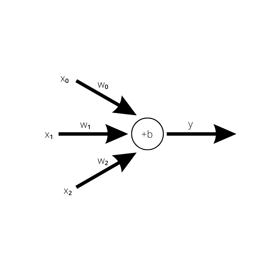
From the above image, we can establish a mathematical definition using the following function:

$$f(x) = b + \sum_{i=0}^{2}x_iw_i$$

Generalizing this definition for $n$ inputs, we would obtain the following:

$$f(x) = b + \sum_{i=0}^{n-1}x_iw_i$$

Here, $x_i$ represents the inputs that are multiplied by their respective weights $w_i$, and then the value $b$ is added to them. Therefore, the parameters to be learned are $b$ and all the weights $w_i$. Normally, a vector notation is used to express the perceptron, where both inputs and parameters are represented as vectors. The notation used for the perceptron in Figure 1: Perceptron with 3 inputs would be as follows:

This representation has a peculiarity. The first input, with a value of $1$, is fixed and is not considered a proper input. It is represented this way to be able to directly add the product of the two final vectors to the value of $b$. The generalization of this definition for $n$ inputs is simple from this example. Simply the inputs and parameters must be added to their respective vectors, without forgetting to include $1$ and $b$ at the beginning of the vectors.

Furthermore, this representation is very useful when there are several perceptrons in the same layer, since by representing the parameters of each one in a vector, all vectors can be combined into a matrix. For example, consider a layer with three perceptrons and three inputs. We could represent them as follows using matrices:

In Figure 3: Matrix representation of the perceptron layer, the weight $w_{ij}$ refers to weight $i$ associated with perceptron $j$. It is important to note that the input remains constant regardless of the number of perceptrons in the layer. To obtain the outputs, it is only necessary to perform a matrix multiplication, which consists of multiplying one by one each element of the parameter vectors with the input vector. Figure 4: Matrix representation of the layer output illustrates what the output would be like using the same representation.

Matrix multiplication is performed in practice by applying the formulas shown in Figure 5: Direct output formulas. These formulas represent the direct process for calculating the output of a 3-input perceptron layer.

The learning process of perceptrons is quite simple. They compare the output obtained by the perceptron with the expected output and use the difference between them to adjust the weights. However, the main problem with perceptrons lies in their totally linear nature, which becomes evident when representing them using vectors and matrices. To overcome this limitation, an activation function is applied to the output of the perceptron, which introduces non-linearity into the process.

When dealing with images, new challenges arise. Images are represented by matrices, where each position corresponds to a pixel and each matrix indicates the intensity of a color or other attributes related to that pixel. However, perceptrons cannot directly process these matrices, as they need to be converted into vectors. However, this conversion implies the loss of information about the spatial arrangement of pixels and their relationship to each other. Elements that were contiguous in the matrix may be very far apart in the resulting vector. This spatial information is crucial for image processing (and chess), so an alternative method is needed.

Fortunately, there is a highly effective procedure known as convolution, which addresses this problem. Convolution allows preserving the spatial structure of images when processing them, which is fundamental for tasks such as object recognition and feature extraction.

Convolution

Convolution is similar to the operation of a perceptron, but operates on square regions (on exceptional occasions rectangular sections can be used) of an image. To better understand how a convolution layer works, it is useful to use an example. In Figure 6: Convolution example, the initial configuration of the input and convolution parameters is shown.

In this example, we will use a stride (displacement) with a value of 1 and a value of $b=1$ (which is added similarly to perceptrons). With the current configuration, a total of 4 convolutions will be performed. In Figure 7: Convolutions performed in the example, it is shown how the convolutions would be carried out.

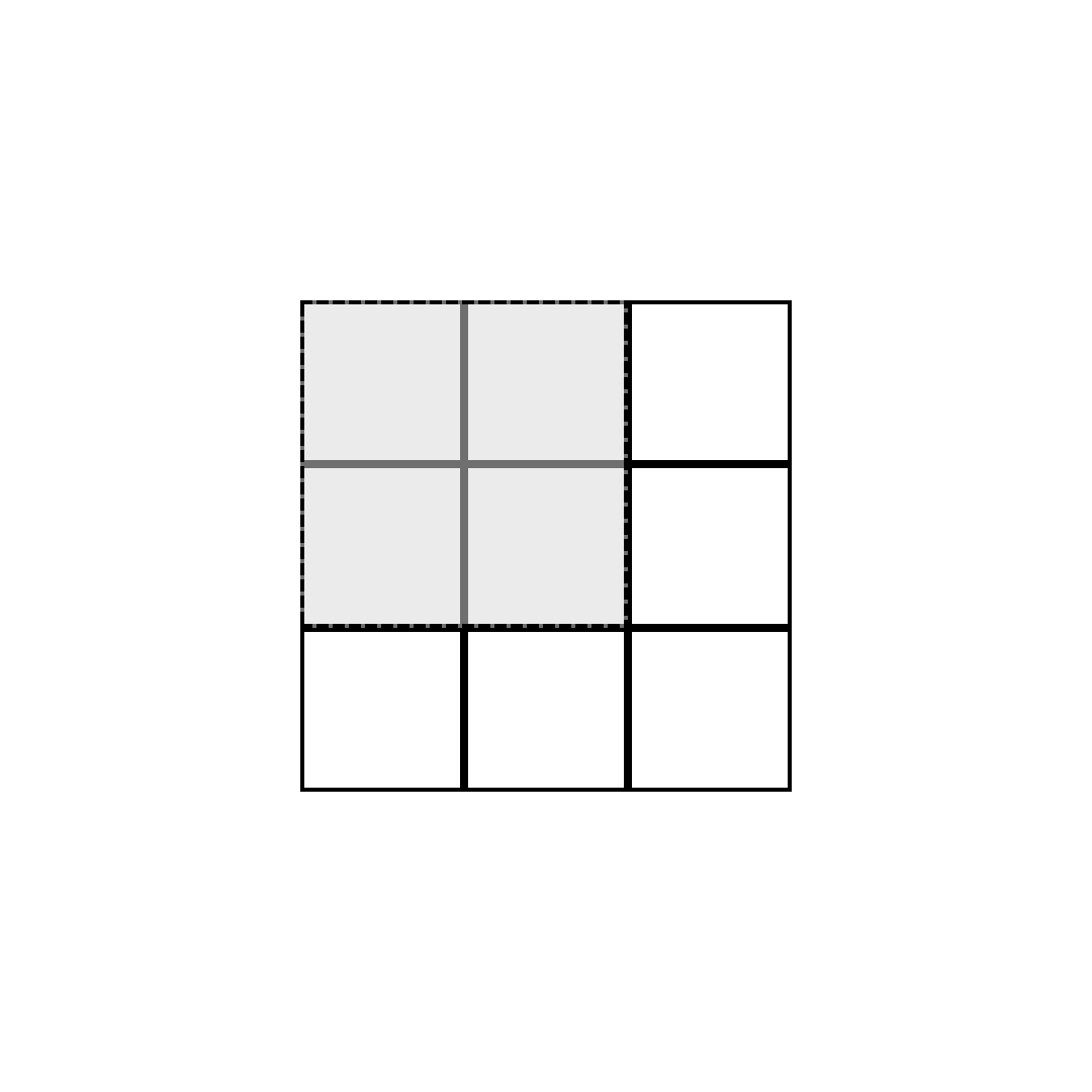
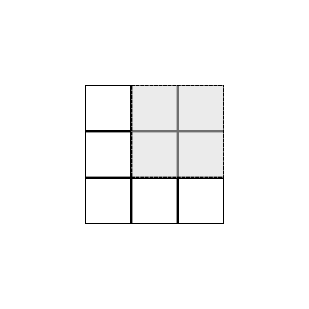
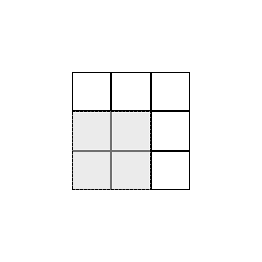
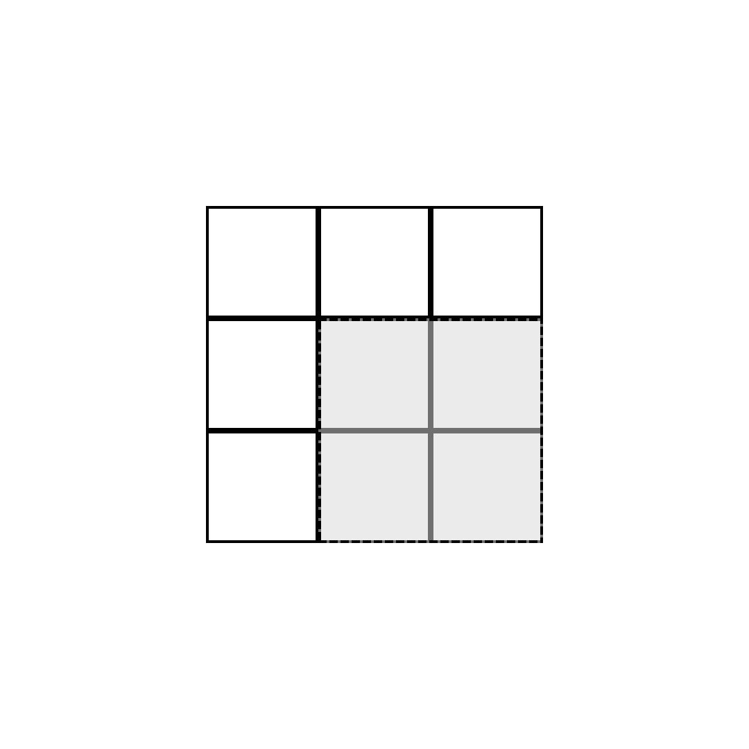
Since four convolutions will be performed, the resulting output will be a matrix of size $2 \times 2$. To obtain the result of each convolution, the input (the shaded region in each convolution) is multiplied by the corresponding convolution parameters. Then all these results are summed and $b$ is added, which will be the output value for that specific convolution. Figure 8: Output of the example convolution shows the output obtained by applying the convolution.

In the detailed analysis of the convolution operation, we observe that the component located at the upper left vertex of the result is determined through a specific calculation: the sum of the multiplications of each element of the convolution kernel with the corresponding pixel of the input image is performed. To exemplify, let us consider the following values: $0.24, 0.12, 0.13, 0.13$, which are multiplied respectively by $0.56, -0.54, 0.07, 0.32$ to then be summed together and finally a constant $1$ is added, the bias term denoted by $b=1$. Thus, the calculated value for the component in the upper left corner is $1.12$.

An important parameter in the convolution process is called padding. This procedure implies increasing the size of images through the addition of zeros at the edges of the image. The utility of this technique lies in its ability to allow performing convolutions more effectively and accurately in the peripheral regions of images, especially near the corners.

In conjunction with convolution operations, a pooling layer is commonly used in convolutional neural networks. This layer plays a crucial role in decreasing the size of the output while preserving, at the same time, the most significant information. Despite its similarity with convolutions, in selecting blocks from the input, the pooling layer is distinguished by not having its own parameters to learn. There are mainly two types of pooling operations: max pooling, which selects the maximum value from the input block, and average pooling, which calculates the average of all values in that block. Both pooling methods consist of converting, in practice, a set of pixels (such as those grouped in squares of 4, 9, 16, among others) into a single pixel, thus achieving a reduction in complexity.

Activation Functions

Activation functions play a fundamental role in expanding the capabilities of neural networks in various domains, by providing them with non-linear characteristics, which are necessary in most problems. These functions generally do not require parameters and three of the most relevant are ReLU, Sigmoid, and Softmax.

ReLU (Rectified Linear Unit) is widely used in the intermediate layers of neural networks, that is, in all layers except the last. Its operation is quite simple. If the input is positive, it remains unchanged, but if it is negative, it becomes zero. Mathematically, it is defined as follows:

$$f(x) = \begin{cases} x, \text{if } x \ge 0 \\ 0, \text{if } x < 0 \end{cases}$$

It is commonly recognized that the use of ReLU, following convolution operations, provides good results. By default, this layer is implemented in the intermediate stages of the neural network (all layers except the last). For the last layer, it is preferable to use different types of activation functions that limit the range of possible values to a more reduced subset. Some of the most prominent are the Sigmoid, Softmax, and hyperbolic tangent functions. The latter will be analyzed in detail in the chapter dedicated to AlphaZero. These functions restrict values to be between 0 and 1 for Sigmoid and Softmax, and between -1 and 1 for hyperbolic tangent.

The Sigmoid and Softmax functions share a common purpose: transforming the output into a probability distribution (Sigmoid can also be used for regressions in the interval $(0,1)$). The difference lies in the fact that the Sigmoid function is applied to a single perceptron, while the Softmax function can be applied to two or more perceptrons. Therefore, Sigmoid is useful for binary decisions (for example, determining whether an object belongs to a category or not), while Softmax can be generalized to as many categories as desired. Therefore, the choice between both will depend on the number of categories that need to be classified.

The Sigmoid function is mathematically defined as follows:

$$f(x) = \frac{1}{1 + e^{-x}}$$

Regardless of how large or small the value of $x$ is, it will never exceed the limits of 1 and 0 respectively. If $x$ equals 0, the result will be $1/2$, so all positive values will be in the interval $(\frac{1}{2}, 1)$ and negative ones in $(0, \frac{1}{2})$.

On the other hand, the Softmax function allows transforming a set of values into a probability distribution, such that the higher values have a greater probability of occurring than those with lower values. This transformation is performed through the use of the exponential function. The mathematical definition of Softmax is:

$$f(x_i) = \frac{e^{x_i}}{\sum_{i=1}^{n}e^{x_i}}$$

The denominator in this fraction corresponds to the sum of all input values $x_i$, each raised to the power of $e$, while the numerator corresponds to the individual value $x_i$, also raised to $e$.

To illustrate the operation of the Softmax function, let us consider the following vector:

$$\begin{bmatrix} 1 & 4 & 3 & 1 \end{bmatrix}$$

First, the common denominator for the four elements is calculated, which turns out to be 80.12. Then, each element of the vector is processed individually, obtaining the following results:

$$\begin{bmatrix} 0,034 & 0,681 & 0,251 & 0,034 \end{bmatrix}$$

As can be observed, the element with value 4 in the original vector is the one that predominates with a probability of 0.681 of occurring. It is also important to note that the sum of all elements is 1, corroborating that the Softmax function has converted the original vector into a probability distribution. Softmax is frequently used in multiclass classification problems (more than two classes) and in situations where an action needs to be selected in a non-deterministic manner.

Backpropagation

Backpropagation is the algorithm that facilitates the calculation of the required updates for all parameters of a neural network. As mentioned earlier, when there is only one layer, calculating the weight updates is quite simple. However, when the number of layers increases, this process becomes more complex. Fortunately, the backpropagation algorithm greatly simplifies this task through the use of derivatives.

The operation of this algorithm is based first on the sequential calculation of the neural network’s layers, storing relevant information such as the output of each of these layers. Upon reaching the end, the output obtained from the neural network is compared with the expected output, using a loss function for this purpose. This function will generate a number that will indicate how distant both outputs are; the higher the number, the worse the neural network’s performance.

The next step is “propagation backwards”, which is the essence of the algorithm. Starting from the loss, each layer is traversed starting from the last, modifying the neural network’s parameters. Within this process there is a sub-algorithm called optimizer, whose objective is to minimize the loss function.

The loss function has two parameters: the expected output $y$ and the output generated by the neural network $\hat{y}$. The mathematical definition of the loss function would be:

$$f(\hat{y},y) = \alpha$$

Where $\alpha$ represents the value corresponding to the loss. However, the inputs to the loss function can be heterogeneous, and may even be of different types. A common scenario is when the neural network’s output is a probability distribution, while the expected output is simply a number indicating the action; in such case, the probability of executing that action according to the probability distribution will be chosen.

The choice of loss function is closely linked to the type of problem being solved. Thus, if the problem is classification, the loss function will be very different from the one that would be used in a regression problem.

The optimizer seeks to minimize the loss function, acting as a kind of “guide” for the neural network. The usual method to achieve this is gradient descent, which aims to find the minimum values of a function, in this case, the loss function. The optimizer uses gradient descent along with the modification of other parameters, mainly the learning rate (which indicates how much the neural network’s parameters are modified) to optimize performance.

Among the optimizers available for neural networks, one of the most used is SGD (Stochastic Gradient Descent). This algorithm implements a version of gradient descent that introduces random variations with the purpose of avoiding being trapped in local optima. Local optima are points where the function reaches a minimum value in a specific region of the search space, but which do not necessarily represent the global minimum value of the function. These local optima can limit the optimizer’s ability to find the most optimal solution, hence the importance of having strategies to avoid them.

SGD solves this problem by introducing an element of randomness into the gradient descent process. Instead of using the entire data set to calculate the gradient at each step (as is done in standard gradient descent), SGD selects a random subset (or even a single example) to make the calculation. This introduces variability that can help escape local optima.

Another notable optimizer is Adam (Adaptive Moment Estimation), which is an extension of SGD that introduces several improvements. The first of these improvements is the use of adaptive learning rates, which means that Adam adjusts the learning rate (the size of the steps taken in gradient descent) for each parameter individually based on estimates of the first and second moment (that is, the mean and variance) of the gradients.

Furthermore, Adam also includes a mechanism known as “momentum”, which makes the optimizer not only take into account the current gradient, but also the gradients from previous iterations. This can help accelerate the algorithm’s convergence and also overcome local optima and flat zones of the loss function.

Finally, Adam also introduces a bias correction for its estimates of the first and second moment, which helps obtain more accurate estimates at the beginning of training.

These characteristics make Adam a very effective and widely used optimizer in neural network training. However, like any method, it is not a universal solution and may not be the best optimizer for all situations or for all types of neural networks. Therefore, it is advisable to experiment with different optimizers and configurations to find the most suitable option for each specific problem.

Once all the components that constitute deep reinforcement learning have been analyzed, it is possible to delve into the study of AlphaZero and its application in the field of chess. AlphaZero represents the convergence of various previously examined blocks, allowing us to understand how these concepts are applied in this millenary game.