AlphaZero

In this section we will delve into the analysis of a revolutionary module that has transformed the chess landscape as we know it. This module, called AlphaZero, is famous for its impact in the field of computational chess. Although the source code of AlphaZero is not available to the public, the methodology and its functioning have been meticulously described in the research article published by Deep Mind [Silver, 2017].

On the other hand, there exists an open source version This term indicates that the source code is available for consultation and free use, called Leela Chess Zero (LCZero), whose architecture and operating mechanism are remarkably similar to those of AlphaZero.

Both LCZero and AlphaZero operate on the principle of using an artificial intelligence (AI) without prior knowledge of the game of chess, hence the term “Zero” in their respective names. This AI is educated and improved as it plays against itself, which allows dispensing with any inherent human prejudice or bias. This methodology represents a marked contrast with traditional approaches, in which the search for moves is based on knowledge provided by chess experts.

In general terms, both systems consist of two fundamental elements: a neural network and a Monte Carlo search tree. The neural network takes as input a specific chess position and returns, as output, the probability distribution of possible moves and an evaluation of that position, which will be between -1 and 1. The Monte Carlo search tree, using the information provided by the neural network, selects the best move to make in the given position.

The main challenge that LCZero faces compared to AlphaZero lies in its limited computational capacity. To mitigate this problem, the developers of LCZero have implemented a distributed solution, thus allowing any user to contribute to LCZero’s training, contributing their “grain of sand” https://lczero.org/contribute/.

Neural Network Architecture

The neural network in question has a large number of layers, particularly in the feature extraction section. The input consists of a series of channels (8x8 matrices), which take only values 0 or 1. These channels contain the information of the position in a form that is easily interpretable for the neural network. Subsequently, feature extraction is performed; during this process, the neural network identifies and extracts patterns from the input channels. These patterns are then processed by the final layers of the network to determine the value of the current state and the action selection policy.

Figure 1 shows the neural network used by AlphaZero with the aforementioned parts.

AlphaZero neural network

Input

As specified in the research article, the input comprises a total of 119 channels. These channels can be classified into two main groups.

The first group consists of information relating to the arrangement of pieces on the chess board and two additional channels to indicate if a specific position has been repeated once or twice.

To represent the arrangement of pieces, the format known as one-hot encoding is used. In this format, all elements of the $8 \times 8$ matrix are initially set to 0 and changed to 1 if a piece of a particular type is found in that square. Thus, each type of piece is associated with a specific channel.

As an illustration, consider the board shown in Figure 2. Below, the channels corresponding to several of the pieces present on this board are shown.

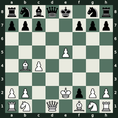
First, we start with the white pawns. Figure 3 shows the resulting matrix. In this matrix, all positions occupied by white pawns are represented with the value 1, while empty positions are represented with the value 0. Each type of piece (pawn, knight, bishop, rook, queen and king of both colors) is assigned to a specific channel, giving a total of 12 distinct channels.

In the following case, we proceed with the black knights. Figure 4 illustrates the channel corresponding to this piece.

Similarly, the process would proceed with the rest of the types of pieces. Continuing with the channels, it is pertinent to discuss the two channels used to report position repetition. The first channel will have all its values at 1 only if the position has been repeated once, while the second channel will be activated if the current position has been repeated exactly twice. This provides the neural network with the information that if it repeats the position one more time (having been repeated a total of three times), the game will be declared a draw. In total, this first group of channels has $12+2=14$ channels. This group is repeated 8 times, since the last 8 positions are stored instead of only the last one In my opinion, I do not consider it necessary to store the last 8 positions, with only the last one being necessary, since the information from the first two groups of channels provides all that is necessary for the current position. Thus, there will be $14*8=112$ channels in total.

In addition, the possibility of en passant must be taken into account. To represent this eventuality, the pawn that can be captured en passant is moved from the fifth row to the last row in its corresponding channel. Since a pawn can never be on the last row, this representation does not generate any confusion.

On the other hand, the second group of channels stores information relating to the current position that is not directly related to the arrangement of pieces. This group consists of 7 channels, adding a total of $119$ channels when combined with the first group. Below are the channels of this second group:

• Color: Indicates the player’s turn. If it is White’s turn, all channel values will be 0; otherwise, they will be 1.
• Number of moves: Represents the total number of moves made in the game. All values in the matrix will correspond to this number. For example, if 49 moves have been made, all values in the matrix will be 49.
• White kingside castling: Indicates if White can perform kingside castling. If possible, all channel values will be 1; otherwise, they will be 0.
• White queenside castling: Similar to the previous one, but for queenside castling.
• Black kingside castling: Similar to the previous one, but for Black and kingside castling.
• Black queenside castling: Similar to the previous one, but for queenside castling.
• Number of moves without progress: Similar to the number of moves channel, but counts only those in which no progress has occurred. A move is considered to produce progress if a pawn advances or a piece is captured. If 50 moves are made without progress, the game will be declared a draw.

Thus, the input to the neural network will consist of 119 matrices of $8 \times 8$. Additionally, it is relevant to note that the board is always presented from the perspective of the player who has the turn, that is, not all players will see exactly the same board, but one of them will perceive it rotated.

This input undergoes a convolution layer, inaugurating the feature extraction phase. Each convolution layer is formed by convolutional filters, which are complemented by batch normalization and a ReLU activation function. This scheme is consistent throughout all the convolutional layers of this neural network.

Batch normalization is a technique that normalizes the input. Its use is very common, as it tends to improve the stability and performance of neural networks [Ioffe, 2015]. To apply it, the mean and standard deviation of the input are calculated. Then, the following formula is applied to each input value ($x_i$):

$$y_i = \frac{x_i-\mu}{\sigma}$$

Where $\mu$ is the mean and $\sigma$ is the standard deviation.

In a more complete variant of batch normalization, two additional parameters are included that allow scaling and shifting the normalized output ($y_i$). Thus, the final result ($z_i$) is calculated as:

$$z_i = \gamma*y_i + \beta$$

In this case, the learnable parameters are $\gamma$ (scale) and $\beta$ (shift).

Feature Extraction

The portion of the neural network dedicated to feature extraction is quite voluminous. It consists of a total of 40 residual blocks. Each of these residual blocks includes two convolutional layers, but the second layer has a notable peculiarity. What is special about this second layer is that it has a connection to the original input of the residual block, which is activated after batch normalization in this layer. This residual link allows adding the output, after its normalization, with the original input of the block. This addition operation is performed element-wise. Finally, the ReLU activation function of the second convolutional layer is applied to this result.

Thanks to this residual connection, backpropagation can be performed more directly, without needing to pass through all intermediate layers.

Figure 5 illustrates the structure of a residual block as described above.

Structure of a residual block in AlphaZero

Policy

The process begins with feature extraction, which is subsequently channeled through a series of convolution filters. Batch normalization is applied to this data, followed by the implementation of a ReLU activation function. At the end of this process, we obtain a tensor (several ordered matrices) of dimensions $8 \times 8 \times 73$. This tensor reflects the probability distribution of the different possible moves on a chess board, obtained after applying the Softmax function.

Although at first glance, $8*8*73=4672$ may seem like an exorbitant amount of possible moves, this figure is due to the fact that it includes all combinations of squares and feasible moves in the game, and even some more. Each component of the $8 \times 8$ tensor corresponds to a specific square on the chess board where a piece that is about to move is located. More specifically, there are really 73 possible moves.

Within these 73 possible moves, the first 56 correspond to queen moves, including all possible moves for the queen, king, bishop and rook. The next eight moves, that is, those from 57 to 64, encompass the eight possible knight jumps. Finally, the remaining 9 moves are reserved for situations where a pawn is promoted to a piece other than a queen.

The logic behind queen moves is governed by the orientation of a compass; consequently, the queen can move in any of the 8 directions indicated by it. In each direction, the queen has the ability to move between 1 and 7 squares. The product of these values provides us with the total number of possible moves for the queen. During encoding, each direction will be assigned a numerical value between 1 and 7, as shown in Figure 6. To this value will be added the number of squares that the queen plans to move.

Assignment of values to the directions of queen movements

The formula will therefore be as follows:

$$f(\alpha_d,c) = 7*\alpha_d + c$$

$\alpha_d$ is the coefficient of the directions (see Figure 6) and $c$ the number of squares to move.

Below is an example to clarify the operation.

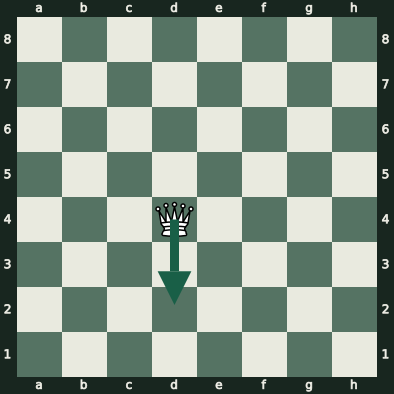
The queen aims to move to the square indicated by the arrow, specifically, from d4 to d2. This move, which is made in a southerly direction, has an assigned coefficient of 4. Thus, the resulting action will be $4*7+2=30$ in the case that the move covers two squares. In relation to the coordinates of the 8x8 subsection, we would be talking about $(4, 4)$, since it is located in row 4 and in column “d”, which has a numerical value equivalent to 4.

In the case of knight moves, the process is similar. The criterion of clockwise direction will be applied again, so the squares located in the upper right corner will receive values of 1 and 2. The corresponding formula would be:

$$f(\beta_s) = 56+\beta_s$$

In this formula, $\beta_s$ denotes the coefficient of the knight jump according to the clockwise direction. To this coefficient is added $56$ to indicate a knight move.

Figure 7 provides an illustrative example of this encoding scheme.

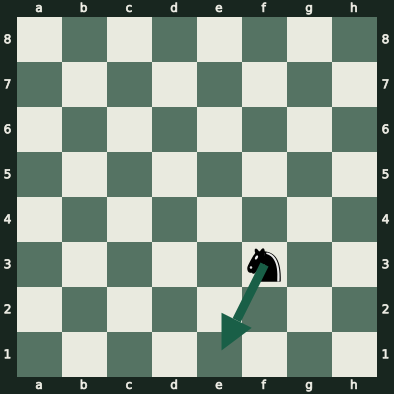
In the example, the knight located on square f3 intends to move to square e1. This move is identified by a coefficient of 5, being the fifth jump in a clockwise direction, so the action will be computed as $56+5=61$. The corresponding coordinates would be $(3, 6)$ because the knight is located on square f3 (row 3, column 6).

Finally, pawn promotion must be considered. A pawn can become a queen, knight, bishop or rook once it reaches the last rank. If it transforms into a queen, its move is encoded normally as such. However, if it promotes to any of the other three pieces, it needs its own move code. Additionally, when a pawn promotes, it can do so by advancing one step on the upper left diagonal, one step forward, or one step on the upper right diagonal. That is, there will be $3*3=9$ possible moves in total. An analogous procedure to queen moves will be applied, where a coefficient will be assigned to each promoted piece and then the move will be added. The coefficients to be used are:

• Rook: 0
• Bishop: 1
• Knight: 2

Regarding the moves, the following values will be assigned:

• Upper left diagonal: 1
• Step forward: 2
• Upper right diagonal: 3

The formula to be applied will be:

$$f(\delta_p,m) = 64+3*\delta_p+m$$

Where $\delta_p$ is the coefficient of the promoted piece and $m$ the value of the corresponding move. One is subtracted from the original value.

Below is an example of pawn promotion. Figure 8 represents the initial position.

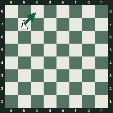
In this case, the pawn aims to promote to a bishop, so the coefficient $\delta_p=1$. Applying the formula, we obtain that the action is $64+3*1+3=70$ (considering a move towards the upper right diagonal).

A possible question could be: how are promotions represented on the black pieces side? However, this would not be necessary since the board is always visualized from the player’s perspective, so pawns would always promote on the last rank.

This representation, however, presents a problem. Many of the actions cannot occur in all positions. For example, if you have a queen located in the lower left corner (square a1) it can never move to the southeast, south, southwest, west and northwest. In the case of a knight on that square, it could only move to 2 of the 8 possible squares. Additionally, a pawn can only promote if it is on the penultimate rank. Taking these factors into account, Leela Chess Zero was able to reduce the total number of moves to $1858$ [Leela Chess Zero developers]. To achieve this, the same system as before is followed, but all impossible moves are eliminated.

Value

Fortunately, the mechanism of the value output is considerably simpler than that of the policy. The process begins with the application of a convolutional filter, followed by batch normalization, and then a ReLU activation function is implemented. From this point, we transition from two-dimensional matrices to a vector, initiating the application of a perceptron layer. Then another ReLU activation function is implemented, followed by another perceptron layer consisting of only one perceptron. To the output of the latter, an activation function known as Tanh is applied.

The Tanh activation function has the special characteristic of transforming all values to the range $(-1,1)$. The mathematical definition of this function is as follows:

$$tanh(x) = \frac{e^x-e^{-x}}{e^x+e^{-x}}$$

This function is ideal in relation to the expected reward which is also within this range. Thus, values close to -1 indicate a position on the verge of defeat, if it is close to 0 it is interpreted as an even position, and finally, if its value approaches 1, victory is practically assured. In case this function receives a very high positive value, it will return a value close to 1, while if this high value is negative, the result will be close to -1. These expected rewards will always be evaluated from the player’s perspective, so that if you have the advantage, the rewards will be greater than 0 for both white and black pieces.

Monte Carlo Tree Search

The Monte Carlo Tree Search (MCTS) is one of the most outstanding aspects of AlphaZero. This tree search mechanism follows logic similar to the Minimax algorithm and its improved version with alpha-beta pruning, but introduces the component of simulations.

When the artificial intelligence is in a particular state, it generates a tree similar to the previously mentioned algorithms, although this will be much smaller. This tree will comprise the states that result from taking an action in the original state, and in turn the states that arise from taking actions in the previously generated states. This process concludes when a leaf node of the tree is reached. Each node of the tree preserves the following information:

• $N$: The number of times that action has been selected in the simulations.
• $W$: The cumulative value of this state according to the simulations.
• $Q$: The average value of this state based on the simulations. It is obtained by dividing the total value by the number of times that action has been selected. In other words, $Q = W / N$
• $P$: The initial probability of selecting that action (provided by the policy of the neural network).

The simulation process is performed a certain number of times, which can be defined by available time (for example, all possible simulations in one minute) or by a fixed number of simulations. When selecting the action to take, three parameters are considered: $Q$, $N$ and $P$. The higher the values of $Q$ and $P$, the more likely the simulation is to be selected; however, in contrast, it is desired that $N$ has the lowest possible value to maximize the function. $N$ operates in this way to facilitate exploration of those nodes that have not yet been sufficiently explored. The formula to obtain the value of the action would be as follows:

$$A = Q + \frac{P}{1+N}$$

As can be seen, increasing $Q$ and $P$ increases the value of $A$, while increasing $N$ decreases the value of $A$. $1$ is added to $N$ to avoid divisions by zero ($N$ can have a value of $0$).

In a given node, the action that leads to the state with the highest value $V$ will be selected. This process ends upon reaching a leaf node, initiating the update phase. The value of the leaf node $v$ is obtained using the neural network and the following updates are carried out in all the nodes that have been visited:

$$N := N + 1 \\ W := W + v \\ Q := \frac{W}{N}$$

On one hand, the number of simulations performed on that node is increased. The total value $W$ is increased by adding the value obtained in this simulation, and the value of $Q$ is recalculated with the updated values of $W$ and $N$.

Once all simulations have finished, the best move is selected according to them. To do this, the action that has had the largest number of simulations is chosen, that is, that has a higher value of $N$. This is the competitive strategy (which seeks to play in the best possible way), but it may be that the system is in training and has greater interest in exploring (thus resurfacing the dilemma of exploration versus exploitation). In this last case, the system will generate a probability distribution based on the $N$ of the different nodes. To generate the probability, it simply adds all the simulations and divides the simulations of each node by this total. After choosing the action, the entire tree is discarded except for the subtree corresponding to the selected action, this allows reusing the calculations made in the previous step to calculate the following moves. [Silver, 2017] [David Foster].

Below is an illustrative example that aims to clarify the functioning of the Monte Carlo tree search.

Consider the position shown in Figure 9, where White must choose between three possible moves: Kf3, b3 and Qb3.

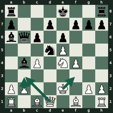
The agent playing with the white pieces has generated a Monte Carlo tree search, and is about to carry out the last simulation of the tree. The node only shows the values $N$, $W$ and $P$, since $Q$ can be easily calculated from $W$ and $N$.

State of the MCTS tree before performing the last simulation

The last simulation is performed, selecting the moves Kf3 and f5, since they are the ones that present the highest value according to the formula used for simulations. Upon reaching the node after f5, the neural network is executed, obtaining a value of $v=0.6$. With this value, we proceed to update all the nodes that were traversed during the simulation, resulting in the following tree:

State of the MCTS tree after finishing the last simulation

Once the last simulation has been completed, it is time to select the action to carry out. The criterion for selection is based on the number of simulations $N$, so the selected action is Kf3. After this decision, the entire tree is discarded except for the part that originates from the node to which the move Kf3 has led.

After having studied the functioning of the Monte Carlo tree search, the next step is to examine how the artificial intelligence was trained and evaluated.

Training

The training process of the neural network starts from scratch, without providing it with any pre-existing knowledge about chess, making it a tabula rasa. Its only option to acquire knowledge is to play games against itself, learn from its own mistakes and, in this way, gradually improve its performance.

There are significant differences in AlphaZero’s learning compared to its predecessor, AlphaGo Zero. In the case of AlphaZero, the neural network parameters are constantly updated, regardless of the results. In contrast, AlphaGo Zero only updates its parameters if the most recent neural network manages to surpass its previous version.

During the training process, AlphaZero generates a large number of games against itself. These games become the training corpus of the neural network. All positions in these games are randomized and, for each one, the search probabilities corresponding to the Monte Carlo tree search are stored, as well as the result of the game. Subsequently, the neural network receives each position and returns both the policy (search probabilities) and the value of the state (result of the game).

To evaluate the network’s performance, two metrics are used: the Cross-Entropy Loss function to compare the policy returned by the network with the stored one, and the Mean-Squared Loss function to compare the state value. With these two functions the total loss is obtained.

Finally, in order to prevent overfitting Overfitting occurs when a neural network model is excessively trained with a specific dataset, which leads to learning patterns that are specific to that data but do not generalize well to new data. This can result in poor performance when the model is applied to new samples., a regularization component is introduced in the calculation of the total loss.

Cross-Entropy Loss

The Cross-Entropy Loss function is commonly used in classification problems or in determining the policy of actions. This function assumes that the output of the neural network is a probability distribution, while the actual or expected output is a vector in one-hot encoding format. For example, if we have a total of 5 possible actions and the chosen action is the third, the vector in this format would be as follows:

$$\begin{bmatrix} 0 & 0 & 1 & 0 & 0 \end{bmatrix}$$

In this vector, all values are zero except in position 3, which corresponds to the selected action and has value 1. This vector and the probability distribution are introduced into the formula of the Cross-Entropy Loss function:

$$\mathcal{L}_1(\hat{y},y) = - \sum_{i=1}^{n}y_i*\log{\hat{y}_i}$$

Here, $y$ represents the vector in one-hot encoding format and $\hat{y}$ the probability vector. [Kiprono Elijah Koech]

An important observation is that, although the vector has $n$ elements, only the value in the position that has a 1 will affect the final result, since when $y_i=0$, the corresponding term in the sum is canceled In the case that $0*\log 0$ is obtained, it is taken by convention to be equal to $0$ to facilitate training. Therefore, this loss function evaluates the probability that the expected action or class occurs. It is important to note that the function will always yield positive values, since the logarithmic term will provide negative values (when receiving values between 0 and 1) that are canceled with the negative sign that precedes the summation.

Mean-Squared Loss

The Mean-Squared Loss function is frequently used in regression problems, like the Cross-Entropy Loss function. In this case, this function is used to approximate the expected reward. Unlike the Cross-Entropy function, its operation is simpler, since it compares the difference between two numerical values using the following formula:

$$\mathcal{L}_2(\hat{y},y) = (\hat{y} - y)^2$$

To calculate this loss, the neural network’s prediction is subtracted from the real value and the result is squared, thus ensuring that the loss is a positive value. If this loss belonged to a batch (that is, in a single pass of the neural network several inputs are calculated), this value would have to be divided by $n$, where $n$ is the number of inputs. The formula would be as follows:

$$\mathcal{L}_2(\hat{y},y) = \frac{1}{n}\sum_{i=1}^{n}(\hat{y}_i - y_i)^2$$

Where $\hat{y}_i$ and $y_i$ correspond respectively to the values of position $i$ in the neural network prediction and the real value [George Seif]. It would be applied in the same way to Cross-Entropy if it were a batch by calculating the average between all.

Regularization

AlphaZero employs a type of regularization known as L2, one of the most used techniques in the field of artificial intelligence. The purpose of regularization is to decrease the complexity of the model and avoid overfitting. To achieve this, an additional term is added to the general loss function, which increases its value as the complexity of the model increases. But how is this complexity measured? Actually, it is quite simple: the weights of the neural network itself are used. The greater the distance of these weights from zero, the greater the complexity of the model.

L1 regularization calculates the absolute value of the weights, while L2 calculates the square of the weights. The formula for L2 regularization is as follows:

$$L2(w) = \alpha*\sum_{i=1}^{n}(w_i)^2$$

In this formula, $w$ represents all the weights of the neural network and $\alpha$ is a regularization parameter with a very small value, typically 0.01 or 0.001, or even smaller. The total loss of the model, which is used for backpropagation to calculate the update of the neural network weights, is obtained by adding the two loss functions described above and the L2 regularization term [Anuja Nagpal].

Overfitting occurs when the model fits very well to the training data, but has poor performance in generalization for new or previously unseen inputs. Since overfitting indicates that the model is too complex, regularization can be an effective method to mitigate this problem.

Therefore, the total loss of the model is calculated as follows:

$$\mathcal{L} = \mathcal{L}_1 + \mathcal{L}_2 + L2$$

Evaluation

After the completion of the neural network training process, it becomes essential to evaluate its performance compared to that of humans and other computer programs. However, considering that in the game of chess, computer programs have far surpassed human players for many years, the benchmarking of our network will therefore only be done against computer programs.

Along these lines, the AlphaZero team opted to contrast its performance with the program that was proclaimed champion of the Top Chess Engine Championship (TCEC) in 2016. This program is known by the name of Stockfish, and was characterized at that time by having an architecture based on the alpha-beta pruning technique and a series of highly complex heuristics.

In the confrontation consisting of a total of 100 games, AlphaZero achieved an impressive record of 28 wins and 72 draws against this formidable rival. These excellent results caused an unprecedented revolution in the field of chess programs, highlighting the potential of artificial intelligence and neural networks in the domain of this millenary strategy game.

Implications

The most notable change that has occurred in the field of artificial intelligence was the transition from the use of heuristics designed and coded by humans to the adoption of heuristics generated through neural networks. This transformation marked a turning point in how machines learn, interpret and make decisions based on the data they process.

This change, however, had the consequence that modules that still used the old heuristics were at a disadvantage compared to those that had incorporated the new technology. These older modules, which once dominated their respective fields, lacked the ability to compete effectively with modules based on neural networks, resulting in considerable disparity in terms of efficiency and precision.

However, it is important to note that many of these systems based on traditional heuristics have been able to adapt to this new era of machine learning. A notable example is that of the chess program Stockfish. This chess engine, which once relied on manually designed heuristics, has successfully integrated a neural network into its architecture, which has considerably boosted its performance. This adaptation has not only allowed Stockfish to remain competitive against its neural network-based contemporaries, but has also demonstrated the versatility and inherent adaptability of these systems. We will see in more detail how Stockfish managed to integrate neural networks in the next chapter.