Alpha-beta pruning

Alpha-beta pruning is an efficient technique that drastically reduces the number of states visited in the game tree of the minimax algorithm. Its main objective is to avoid exploring branches of the game tree that will not lead to better results than those already found. This strategy is divided into two variants: alpha pruning, applied at maximization levels, and beta pruning, used at minimization levels.

To implement alpha-beta pruning, two values are employed: alpha ($\alpha$) and beta ($\beta$). The alpha value represents the best result obtained so far during the maximization phase, while the beta value fulfills the same function in the minimization phase.

Alpha and beta values are transmitted from parents to children in the game tree, but not in the opposite direction. Additionally, alpha and beta values can also be inherited between siblings.

In the context of alpha-beta pruning, a state is considered the parent of another state if the first is at the level immediately above the second and there is a link connecting them. Conversely, a state is said to be the child of another state if the child is at the level immediately below the parent and there is a link between them. The concept of sibling is closely related to these two relationships. A node (state) is said to be the sibling of another state if they share the same parent. In trees, by definition, a node can only have one parent.

When calculating the alpha value, the following formula is used:

This formula is executed once for each child of a maximization state. Each time it is executed, the alpha value is updated. Initially, $\alpha = -\infty$ is established, which means that any number will be greater than this value. However, it is important to note that the initial alpha value can be obtained from siblings and the parent, which will be explained in detail in a later example. Therefore, it will not always be equal to $-\infty$.

On the other hand, the formula for calculating the beta value is similar, but in this case the minimum is taken and the alpha values of the children are used:

As with alpha, this formula is executed the same number of times as children a minimization state has. If a minimization state has not inherited the value from its parent or any of its siblings, $\beta = +\infty$ is established. This ensures that any alpha value found in the children will be less than the beta value.

In summary, these formulas allow updating and maintaining alpha and beta values during the search process in the game tree. The alpha formula uses the maximum between the current alpha value and the beta values of the children, while the beta formula uses the minimum between the current beta value and the alpha values of the children. These updates are essential to carry out alpha-beta pruning and optimize the minimax algorithm search in the game tree.

The pruning process occurs as follows: if at any point while exploring the tree, the alpha value is greater than or equal to beta, then we know that the next branches or nodes that were going to be explored in that path will not change the result, since alpha represents the best move that the maximizing player already has guaranteed, and beta represents the best move that the minimizing player already has guaranteed. As a result, it makes no sense to continue exploring that path and it is “pruned”.

Understanding alpha-beta pruning can be challenging without practical examples. Therefore, both a generic example and a specific example related to chess are presented below, with the aim of facilitating understanding of the algorithm.

Generic example

The following example provides an extension to the one presented in the previous chapter, with a subtle but important variant. This time, each node will hold not only its own value, but also a value called $\alpha$ or $\beta$, according to the corresponding alternation between levels: even levels will carry the $\beta$ value and odd levels the $\alpha$ value. Level numbering starts from zero.

This scheme entails a particularity: it will not be feasible to explore the tree level by level as was done in the previous examples, since we will need to reference the $\alpha$ and $\beta$ values of sibling nodes.

Without further ado, the concrete example is presented in the following figure, which we will refer to as the generic alpha-beta game tree:

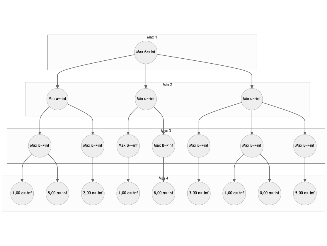
We will begin our exploration from the far left of the tree. Had we opted to start from the right, we would have obtained a slightly different tree, but the evaluation at the final node would have remained invariant. Therefore, both strategies are valid. Likewise, if we alter the order of visitation among sibling nodes, the final result remains, although the number of nodes to process may vary. Unfortunately, determining the optimal order to arrange nodes —so as to minimize the amount of processing— is impossible without developing the tree in its entirety. After the first resolution phase, we will obtain the tree shown in the first alpha-beta resolution phase.

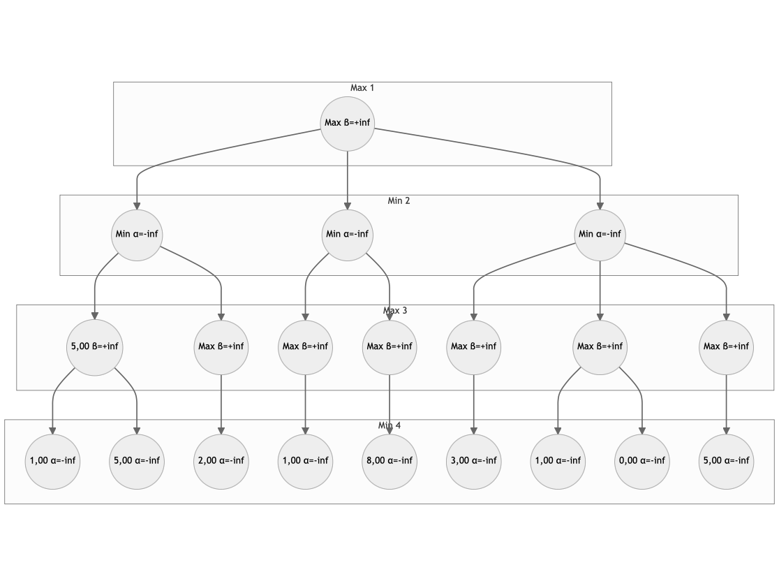
The processed node, which is the first element of level 2, has been assigned a heuristic value of 5. This value is obtained by being the maximum between 1 and 5. Additionally, since the node is a maximization node and is the first node processed at that level, it is assigned a beta value of $+\infty$ (positive infinity). Next, when exploring the sibling node of this one, the tree represented in the second alpha-beta resolution phase is obtained, corresponding to the second resolution phase of the generic game tree with alpha-beta pruning.

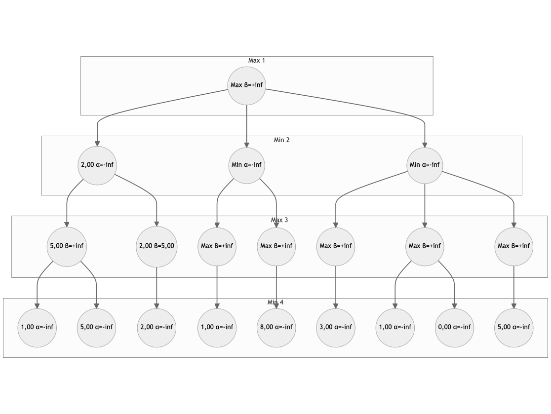
In this case, unfortunately, no significant advantage has been obtained, since the same number of nodes have had to be processed as if the minimax algorithm had been used. This is usually common at the beginning of the tree.

The beta of the sibling of the node processed in the first step has a value of 5, since it has been updated according to the formula and has taken the value of 5 from its sibling. Next, one ascends a level and reaches the parent node of these, which has a value of 2. The $\alpha$ value of this node is negative infinity, since it is the first node processed among its siblings.

In the next phase, the second child of the initial node is processed, as shown in the third alpha-beta resolution phase.

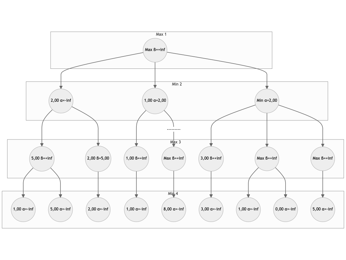
In the initial stage, the left child of the second child of the initial node is processed. This node obtains a value of 1. Since the current $\alpha$ is 2, alpha pruning is activated, which implies that it will not be necessary to process any other child of this node. For this reason, it is not processed and shows that part of the tree with a cut.

The logic behind this pruning is that a value better than 1 cannot be obtained at this node, since being a minimization node, value 1 or a lower one in another child will always be chosen. Furthermore, since the $\alpha$ value is 2 and this is greater than 1, it is not increased.

In the last stage, the rightmost child of the initial node is processed, resulting in the results shown in the final alpha-beta resolution phase.

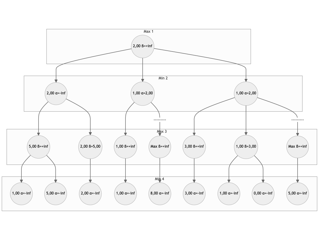
In the first child of the processed node, a beta value of 3 is assigned to its sibling. When exploring the children of that sibling and obtaining values of 0 and 1, the other children continue to be evaluated only if none of them is greater than 3. In this case, since the maximum value obtained is 1 in the central node of the processed node, the beta value is updated to 1.

When ascending to the next level, the value of 1 is received from that node, and since the alpha value is 2 coming from its sibling, alpha pruning is performed and it is not necessary to continue evaluating the other children.

Finally, the value of the initial node is obtained, which is the maximum among the values of its children, resulting in a value of 2. The beta value is $+\infty$ since it has no sibling or parent that establishes a limit value.

Example applied to chess

In the case of chess, the operation of the alpha-beta algorithm is exactly the same as the generic example previously presented. Therefore, in this section we will focus on the implications and importance of the order in which nodes are visited.

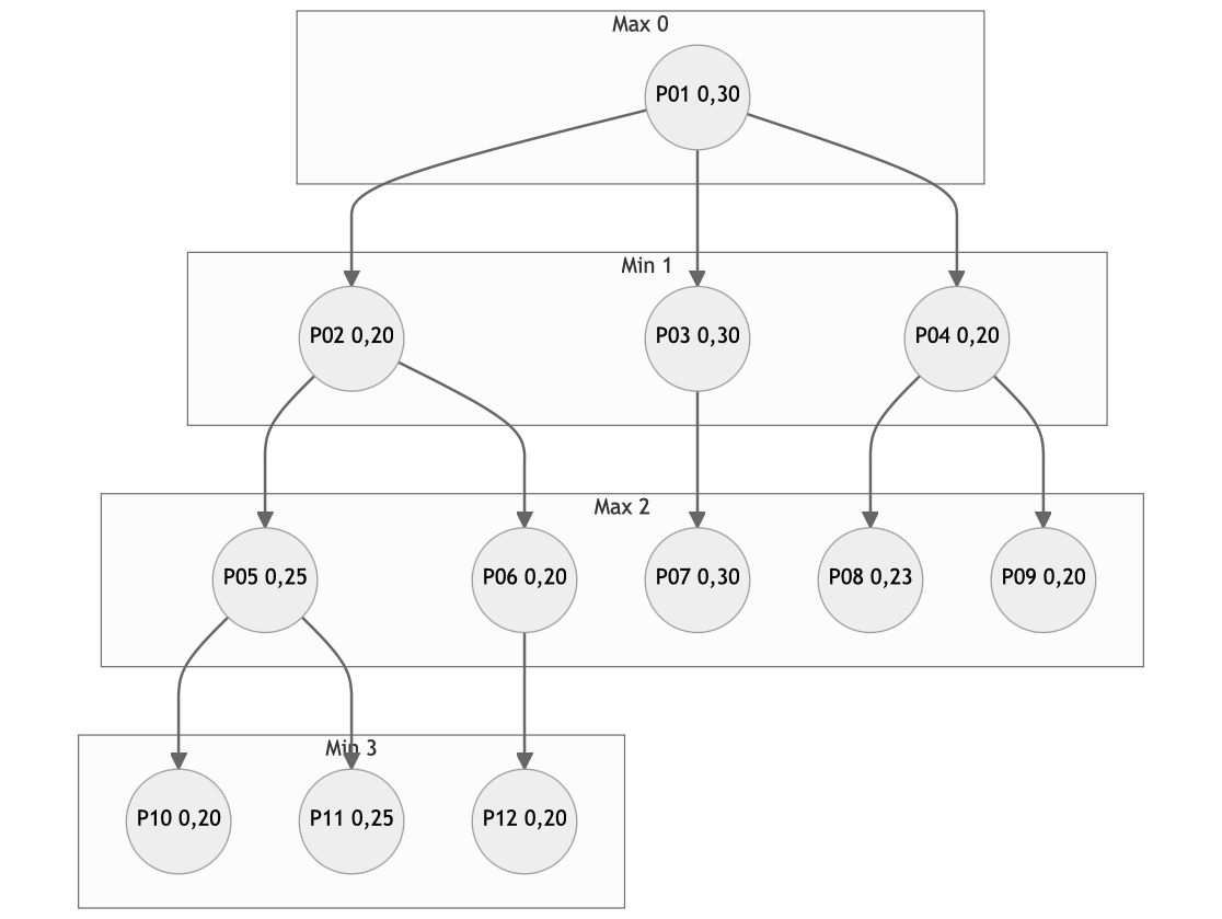
The chess alpha-beta example shows the specific example to be addressed, which is the same one presented in the fourth minimax phase in the previous section, related to the minimax algorithm.

When creating the orders to traverse the trees, it is important to remember two basic rules:

• A node can only be processed if its children have been previously processed.
• If a left-to-right traversal is followed, nodes located furthest to the left that have not yet been processed are processed first, and vice versa.

Next, the usual traversal starting from the left and moving to the right will be used. Therefore, the processing order will be as follows:

The left-to-right chess alpha-beta tree shows the tree using the left-to-right traversal described above.

As can be observed, in this traversal order no node is discarded. This indicates that no improvement would be obtained by using the complex alpha-beta pruning algorithm instead of the simple minimax algorithm.

In the following case, the order will be changed and a right-to-left traversal over the same tree will be followed. Therefore, the new processing order will be as follows:

With the order change, a substantial improvement has been achieved. Now, it is not necessary to visit three of the nodes of the original tree (P05, P10 and P11). This is because when node P02 receives the value from node P06, which is 0.20, it has a higher alpha value, which activates alpha pruning and it is not necessary to generate more child nodes for node P02.

As a conclusion from both examples, it can be stated that alpha-beta pruning can significantly reduce the number of nodes that must be processed. In the last example, 3 nodes are eliminated out of a total of 12, which represents 25% of eliminated nodes. The larger the tree, the greater the percentage of nodes that can be eliminated using this procedure, reaching levels above 50% elimination in some cases.

Another important conclusion is the relevance of the order in which nodes are processed. To select this order, heuristics can also be used, processing first those nodes whose heuristic has a higher value. This can help to further improve the efficiency of alpha-beta pruning by reducing the number of nodes to consider at each level of the tree.