Policy

Policy, in terms of machine learning, represents the decisions made by an agent based on a given state. These policies can be classified in two main ways: deterministic and non-deterministic. The main distinction between them lies in their predictability: a deterministic policy will always result in the same action given the same situation or state, while a non-deterministic policy can lead to different actions even for the same state.

Additionally, policies can also be classified based on the number of possible actions. When this number is finite, we face a discrete action space. In this case, a unique identifier is assigned to each action, usually through an enumeration process. However, it may also occur that the number of possible actions is infinite, and in this case, we would be talking about a continuous action space.

Throughout this text, we will assume that the policy operates on a discrete action space. The analysis and study of continuous action spaces is a topic of great depth and complexity, and falls outside the scope of this book. Furthermore, it has no relation to chess.

Deterministic policies can be represented by the following function:

$$\begin{aligned} f(\alpha) &= \beta \\ \alpha &\in E \\ \beta &\in A \end{aligned}$$

where:

• $\alpha$ represents the current state,
• $\beta$ is the action to be taken,
• $E$ is the set of all possible states,
• $A$ is the set of all possible actions ($A=\{0,1,...,n-1\}$) and
• $n$ is the total number of actions.

Since actions are enumerated from $0$ to $n-1$, any number in that range could be returned by the function. If we have associated values for actions for a particular state, we can create a simple deterministic policy: the action with the highest value will be selected. This policy is called “greedy” because it always chooses the action with the greatest value. This policy is optimal if the values associated with each action are the real ones and not an approximation. However, as we have seen, having these real values in most cases is unattainable.

The structuring of non-deterministic policies is a bit more complex. Instead of returning a single number, these policies return a vector with $n$ elements, where $n$ is the number of actions. The elements of this vector are probabilities, so that the value at position $i$ of the vector represents the probability of choosing action $i$. Being probabilities, the sum of all elements of the vector must be $1$. The function that represents these policies is as follows:

$$\begin{aligned} f(\alpha) &= \Delta \\ \alpha &\in E \\ \Delta &= \{\delta_0, \ldots, \delta_{n-1}\} \end{aligned}$$

where:

• $\alpha$ is the current state,
• $\Delta$ is the probability distribution of actions,
• $\delta_i$ is the probability that action $i$ is selected,
• $E$ is the set of all possible states and
• $n$ is the total number of actions.

After receiving the output of this function, an action is chosen according to the obtained probabilities. This allows the agent to perform a variety of actions instead of always repeating the same one, which can be very desirable when facing human adversaries. As in the case of deterministic policies, if we have the values associated with actions, we can transform them into a non-deterministic policy using the Softmax function (for more details, see the neural networks section). This function, in general terms, creates a probability distribution in such a way that the higher the value of an action, the greater its probability of being selected.

In the case of the 2D game board described in the previous section, there are four possible actions (up, right, down, and left). We enumerate these actions as follows to be able to implement the policies:

$$\begin{aligned} 0 &: \text{Up} \\ 1 &: \text{Right} \\ 2 &: \text{Down} \\ 3 &: \text{Left} \end{aligned}$$

Given the expected rewards (values) shown in Figure 1: Expected rewards for calculating the policy, we can show how a deterministic policy and a non-deterministic policy would select actions.

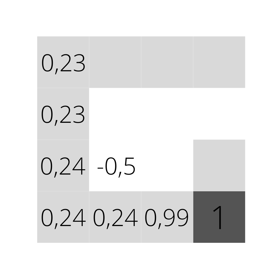
The game piece is located at the initial square (upper left corner) and can perform all four actions. Since squares without any value would have a value of $0$, the deterministic policy would return the value 2, corresponding to moving down. This move would lead to the state with the highest value. Following this procedure, the deterministic policy would continue selecting value 2 until reaching the lower left corner. From that point, it would only return value 1, corresponding to the move to the right, until reaching the final square.

In the case of the non-deterministic policy, the selection of actions would be somewhat more complicated since it requires the use of the Softmax function. When applying this function to the initial square, the following results would be obtained:

$$\{0.2347 \ 0,2347 \ 0,2959 \ 0,2347\}$$

The action of moving right has the highest probability of being chosen, but the other options are not far behind. This is reasonable given that the difference from 0.24 to 0 is minuscule. Non-deterministic policies are usually given a parameter called “temperature”, which allows controlling whether more probabilities are given to actions with higher values or whether all actions have similar probability.

In policy there is a very important dilemma known as the “exploration-exploitation dilemma”. This dilemma arises when the agent must decide between exploring new actions (exploration) or trying to improve known actions with minimal variations (exploitation). If the agent dedicates itself to exploring all the time, the estimates may not be realistic. On the other hand, if it focuses solely on exploitation, it may not find the best solution, since it may be on unexplored paths.

To balance this dilemma, a parameter known as $\epsilon$ (epsilon) is usually used. This parameter indicates the probability of choosing an action randomly. For example, if $\epsilon$ is 0.05, then in 5% of situations the action will be chosen at random. At the beginning, the value of $\epsilon$ will be very close to 1, but it will progressively decrease as more episodes are performed until its value is insignificant or directly 0.

In this way, exploration is encouraged at the beginning of the agent’s training and, as it progresses, it focuses more on improving the estimates for known actions. In the case of non-deterministic policies, $\epsilon$ can be dispensed with and the policy can be configured in such a way that it is interested in actions not taken at the beginning. However, in deterministic policies it is practically mandatory to use this parameter to achieve good performance in policy learning.

Finally, in policy there is a division between whether to use the learned policy for training (on-policy) or to use a different policy than the one used in training (off-policy). The main difference is that in on-policy policies, the policy that is progressively improved is used in the training itself.

In addition to policy, it can also be useful to know the environment’s behavior. For this, the aim is to obtain a “model” of the environment. This model allows knowing how the environment will react to different actions.